ABSTRACT
BHATIA, AMIT. Hierarchical Charged Particle Filter for Multiple Target Tracking. (Under the direction of Dr Wesley E. Snyder.)
Multiple Object Tracking is a significant application of vision-based autonomous solutions. Although it is a logical extension of single object tracking, those algorithms do not simply scale over to the multiple object case. Tracking multiple objects brings on its own set of challenges and complexity.
A multiple object tracking system requires a set of tasks to be completed: (a) Objects need to be detected using Detection algorithms; (b) Objects need to be tracked using Tracking algorithms under conditions of object movement, occlusion, scale changes, illumination changes, scene movement etc.; (c) Such a system must perform as efficiently as possible, with the goal of real time execution. Combining these tasks presents its own set of challenges. This thesis provides a vision based system to track multiple objects under such variety of constraints.
A typical vision-based detection algorithm uses non-uniform convolution as one of its op-erations. This thesis provides a unique method to perform very fast convolution. The method called Stacked Integral Image builds upon the concept of box filters and integral image to accelerate convolution performed in vision based systems.
As tracking algorithms must handle changing scale/size of objects while tracking them, objects can become so small/blurred that geometry based detectors which use corners/edges etc. become unreliable. To utilize radiometric features for object detection, this thesis provides a unique method calledPattern Recognition by Cluster Accumulationthat uses clustering and Hough style accumulation to reliably detect objects when they are small/blurred.
The particle filter is a powerful tool to track an object undergoing non-linear state dynamics with non-Gaussian noise. When tracking multiple objects using multiple particle filters, the particles of non-dominant targets tend to get hijacked by dominant targets. This problem is solved by a new resampling method calledCharged Resamplingwhich uses an electric charge like potential in a probabilistic setting to minimize particle hijack.
To handle moving objects in a moving scene, the problem of double dynamics is solved by employing a layered method called Hierarchical Particle Filter. This method cleanly separates scene tracking from multiple object tracking with a feedback connection to transfer intelligence from one sub-system to another.
c
Copyright 2011 by Amit Bhatia
Hierarchical Charged Particle Filter for Multiple Target Tracking
by Amit Bhatia
A dissertation submitted to the Graduate Faculty of North Carolina State University
in partial fulfillment of the requirements for the Degree of
Doctor of Philosophy
Computer Science
Raleigh, North Carolina
2011
APPROVED BY:
Dr Griff L. Bilbro Dr Christopher G. Healey
Dr Robert St. Amant Dr Wesley E. Snyder
DEDICATION
BIOGRAPHY
The author was born in the city of Kanpur in northern India on August 2nd, 1973. He attended primary and middle schools in the city of Hyderabad and high school in New Delhi. He was admitted to the undergraduate program in Electrical Engineering at the Institute of Technology, in the holy city of Varanasi.
After completing his undergraduate studies in 1995, he joined the information technology company Wipro Infotech in New Delhi where he gained knowledge about data networking products. In 1997 he joined PriceWaterhouse Coopers to become a SAP R/3 consultant.
The SAP skills gave him a job opportunity to move to United States and he joined Dynpro Inc, in Chapel Hill, NC in 1999. He did SAP and E-commerce consulting work at IBM in Raleigh, NC and at Ericsson in Sweden. Going back to his initial love for data networking, the author joined Ericsson IP Infrastructure in 2001 at Raleigh, NC. For the next 8 years, he learned the intricacies of embedded data networking product develeopment from a software perspective.
As the Ericsson office was in NC State University campus, the author decided to pursue his graduate degree and enrolled as a part time student in 2002 in the Computer Science de-partment. After completing his Masters in 2004, he continued on to become a part time PhD student to do research in wireless networks. In 2005, when DARPA announced the Desert Chal-lenge for autonomous vehicles, a small group based in Cary, NC was building an autonomous vehicle. The author volunteered to provide his software skills and the team qualified for the final race in California. Then in 2007, DARPA announced the Urban Challenge for autonomous vehicles. This time, the author provided a complete vision based lane detection and maneuver-ing solution to the NCSU sponsored team, which perfomed fairly well at the race in California. These DARPA challenges sparked an intense interest in this field and the author changed his research field to computer vision.
ACKNOWLEDGEMENTS
I would like to thank my advisor Dr Wesley E. Snyder for his continuous help and direction during this journey. He has a knack of simplifying complex problems into smaller understand-able parts. He encourages to challenge the norm by coming up with simple solutions to hitherto complex solutions/problems. His daily discussions and weekly meetings allowed to keep a con-tinuous drive to speed up the research. His constant guidance was indispensible to complete this thesis.
I would like to thank Dr Griff L. Bilbro for his constant help and suggestions, especially during mathematical situations. The white board discussions with him were invaluable. I would also like to thank Dr Christopher G. Healey and Dr Robert St. Amant for their patience and feedback.
I would like to thank my colleagues at Ericsson for their support and my friends at NCSU for invaluable discussions.
I would like to thank my parents Dr Krishna Gopal Bhatia and Mrs Manju Bhatia for their sacrifices, love, encouragement and direction to help me endure this journey. No words can explain their role in making this happen.
I would like to thank my brother’s family, Mr Aashish Bhatia, Mrs Anu Bhatia, Ms Aakan-skha Bhatia and Mr Akshat Bhatia for their perpetual love and encouragement.
I would like to thank my in-laws, Mr Krishan Kumar Chopra and Mrs Sunita Chopra for their continuous encouragement.
TABLE OF CONTENTS
List of Tables . . . xi
List of Figures . . . xii
Chapter 1 Introduction . . . 1
1.1 Object Tracking . . . 1
1.2 Problem Description . . . 2
1.3 Tracking system compnents . . . 2
1.4 This Thesis . . . 3
1.5 Grants . . . 5
1.6 Appendices . . . 5
1.6.1 Written Qualifier Exam . . . 5
1.6.2 DARPA Urban Challenge . . . 7
1.6.3 Robot Control . . . 7
Chapter 2 Geometric Descriptor Algorithm . . . 8
2.1 Edge Oriented Histogram . . . 8
2.2 Lowe’s Scale Invariant Feature Transform . . . 9
2.2.1 Scale space extrema . . . 9
2.2.2 Keypoint localization . . . 10
2.2.3 Orientation assignment . . . 11
2.2.4 Keypoint descriptor . . . 11
2.3 Mikolajczyk’s Harris Laplace detector . . . 11
2.4 Dalal’s Histogram of Oriented Gradients . . . 13
2.5 Simple K Space . . . 16
2.6 Geometric Descriptor Choice . . . 18
Chapter 3 Radiometric Descriptor Algorithm . . . 19
3.1 Color Histograms . . . 19
3.2 Viola’s Rectangles . . . 20
3.3 New Radiometric Descriptor Developed: PRCA . . . 21
3.3.1 PRCA Overview . . . 22
3.3.2 PRCA Approach . . . 22
3.3.3 Comparison of PRCA with other approaches . . . 29
3.3.4 PRCA Demonstration . . . 31
3.3.5 Performance Comparison of PRCA . . . 34
3.3.6 PRCA as a Radiometric Descriptor: Conclusion . . . 36
Chapter 4 Convolution Algorithm . . . 38
4.1 Background . . . 38
4.2 Integral Image and Repeated Integration . . . 40
4.3 Kernel Integral Image . . . 41
4.4 Stacked Integral Image . . . 42
4.5 Box stack calculation . . . 44
4.5.1 Function Minimization . . . 44
4.5.2 Computational Complexity . . . 45
4.6 Results . . . 46
4.6.1 Finding optimal box sizes and weights . . . 46
4.6.2 Filtering results . . . 49
4.7 Conclusion . . . 54
Chapter 5 Review of Tracking Algorithms . . . 55
5.1 Meer’s mean shift algorithm . . . 55
5.2 Bayesian Filter . . . 57
5.3 Kalman Filter . . . 58
5.3.1 Computational Origin of the filter . . . 59
5.3.2 Discrete Kalman Filter Algorithm . . . 61
5.4 Grid Based method . . . 62
5.5 Extended Kalman Filter . . . 62
5.6 Unscented Kalman Filter . . . 63
5.7 Sequential Importance Sampling (SIS) filter . . . 64
5.7.1 Importance Sampling . . . 65
5.7.2 Use of Importance Density . . . 65
5.7.3 Degeneracy problem . . . 67
5.8 Gordon’s Bootstrap Filter (Particle Filter) . . . 68
5.8.1 Resampling . . . 68
5.8.2 Importance Density . . . 69
5.8.3 Update stage justification . . . 70
5.9 Pitt’s Auxiliary Sampling Particle Filter . . . 70
5.10 Musso’s Regularized Particle Filter . . . 72
5.11 Tracking Algorithm Choice . . . 72
Chapter 6 Review of Visual Detection and Tracking Systems . . . 73
6.1 Birchfield’s color histogram and intensity gradient tracking . . . 73
6.1.1 Gradient Module . . . 74
6.1.2 Color Module . . . 74
6.2 Wren’s Pfinder . . . 75
6.2.1 Person Model . . . 76
6.2.2 Scene Model . . . 76
6.2.3 Analyze new frame . . . 76
6.2.4 Initialization . . . 77
6.3 Avidan’s Support Vector Tracking . . . 78
6.4 Isard’s Condensation Tracking . . . 81
6.5 Isard’s Icondensation Tracking . . . 82
6.6 Meer’s Kernel based Mean Shift Tracking . . . 84
6.7 Duraiswami’s Similarity Measure for mean shift tracking . . . 86
6.8 Yang’s Hierarchical Particle Filter Tracking . . . 88
6.9 Reid’s Multiple Hypothesis Tracking . . . 91
6.10 Cham’s multiple hypothesis figure tracking . . . 95
6.11 Abed’s energetic particle filter for multiple target tracking . . . 97
6.12 Sarkka’s Rao-Blackwellized data association for MTT . . . 99
6.13 Khan’s MCMC based Interacting Particle Filter for MTT . . . 100
6.14 Detection and Tracking System Choice . . . 104
Chapter 7 Initial Detection and Tracking System . . . .105
7.1 Background: ARO Tracking Project . . . 105
7.2 Detection and Tracking System . . . 105
7.3 Simulation Setup . . . 106
7.4 Model . . . 106
7.5 Initialization . . . 107
7.6 Blender loop . . . 108
7.7 Particle filter steps . . . 108
7.7.1 Update . . . 108
7.7.2 New samples . . . 109
7.7.3 Predict . . . 109
7.8 Bounding box . . . 109
7.9 Python script, Simple K Space and Particle Filter . . . 109
7.10 Initial Tracking System Results . . . 110
Chapter 8 Initial System Problem Resolution and Extension . . . .113
8.1 Problems . . . 113
8.1.1 Small size at high elevation . . . 113
8.1.2 Shadow and sun angle . . . 114
8.1.3 Particle Hijack in Multiple Target Tracking . . . 115
8.2 Proposed Solutions . . . 115
8.2.1 Spectral information . . . 116
8.2.2 Charged sampling for Particle Hijack in MTT . . . 118
8.3 Extension . . . 118
8.3.1 Hierarchical PF . . . 118
8.4 Final Proposed System . . . 119
Chapter 9 Particle Hijack and Charged Resampling . . . .121
9.1 Introduction . . . 121
9.2 Bayesian Filter . . . 122
9.4 Particle Filter . . . 124
9.5 Particle Hijack Background . . . 124
9.5.1 Interaction potential and MCMC sampling based tracking . . . 124
9.5.2 Magnetic Inertia Potential Model based tracking . . . 126
9.5.3 Masked Particle Filter based tracking . . . 126
9.5.4 Issues with previous solutions . . . 127
9.6 Proposed Solution . . . 127
9.6.1 Bayesian System . . . 128
9.6.2 Charge force field estimation . . . 128
9.6.3 Probabilistic charged resampling . . . 129
9.6.4 Pseudo code: Probabilistic charged resampling . . . 130
9.6.5 Data Association . . . 131
9.6.6 Occlusion handling . . . 131
9.6.7 Comparison . . . 131
9.7 Results . . . 132
9.7.1 TC1: Regular Sampling: Particle Swap . . . 132
9.7.2 TC2: Regular Sampling: Particle Hijack . . . 132
9.7.3 TC3: Charged Sampling: No Particle Hijack . . . 132
9.7.4 TC4: Charged Sampling: No Particle Hijack (low var) . . . 134
9.7.5 TC5: Charged Sampling: Occlusion: No Particle Hijack . . . 134
9.7.6 Rejection plot . . . 134
9.8 Conclusion . . . 136
Chapter 10 Multiple Object Tracking with Multiple Detectors . . . .137
10.1 Multiple Detectors . . . 137
10.1.1 Model Building . . . 137
10.1.2 Detections . . . 138
10.1.3 Observations . . . 138
10.1.4 Multiple Particle Filter Instances . . . 139
10.1.5 Data Association . . . 139
10.1.6 Charged Resampling . . . 140
10.2 Test Results . . . 140
10.2.1 Static and Crossing Targets with Scene Elevation Change . . . 140
10.2.2 Static and Parallel Interacting Targets with Scene Elevation Change . . . 140
10.3 Conclusion . . . 142
Chapter 11 Hierarchical Multiple Object Tracking System . . . .144
11.1 Hierarchical Particle Filter . . . 144
11.1.1 Background . . . 144
11.1.2 Solution . . . 144
11.1.3 Procedure . . . 144
11.2 Hierarchical Single Target Tracking . . . 145
11.3 Hierarchical Multiple Target Tracking . . . 145
11.3.2 Hierarchical Multiple Target Tracking with targets crossing over . . . 146
11.3.3 Hierarchical Multiple Target Tracking with parallel moving interacting targets . . . 148
11.4 Performance Statistics . . . 148
11.5 Conclusion . . . 152
11.6 Future Research . . . 152
Chapter 12 Novel Contributions. . . .153
References . . . 155
References. . . .155
Appendices . . . .161
Appendix A A-MAC: A More Energy Efficient B-MAC . . . 162
A.1 Introduction . . . 162
A.2 Design . . . 163
A.2.1 B-MAC Overview . . . 163
A.2.2 A-MAC Overview . . . 165
A.2.3 A-MAC-UR: A-MAC for Unintended Receivers . . . 166
A.2.4 A-MAC-HS: A-MAC with Handshake . . . 166
A.3 Power Analysis . . . 167
A.3.1 Notation . . . 167
A.3.2 B-MAC power analysis . . . 169
A.3.3 A-MAC-UR: A-MAC with Destination Layer 2 Address . . . 171
A.3.4 A-MAC-HS: A-MAC with Destination Layer 2 address and Ac-knowledgments . . . 172
A.4 Simulation Results . . . 175
A.5 Implementation . . . 177
A.6 Related Work . . . 179
A.7 Conclusion . . . 180
References . . . 181
Appendix B Lane Detection System for Autonomous Vehicle Navigation . . . 184
B.1 Introduction . . . 184
B.2 Methodology . . . 184
B.2.1 Capture Image . . . 185
B.2.2 Color Segmentation . . . 185
B.2.3 Color Mapping using Munsell Model . . . 186
B.2.4 Recolor Image using Color Histogram . . . 187
B.2.5 Adaptive Scanning to extract single pixel edges . . . 188
B.2.6 Line Detection using Hough Transform . . . 190
B.2.7 Calibration and lane marking generation . . . 191
B.3 Results . . . 192
B.3.1 Platform . . . 192
B.4 Conclusion . . . 195
B.4.1 Current Status . . . 195
B.4.2 Enhancement . . . 195
B.4.3 Future Growth . . . 195
References . . . 196
Appendix C Control of a Ring of Robots with Vision . . . 197
C.1 Visibility . . . 197
C.2 Correction for different camera focal lengths . . . 199
C.2.1 Zoom-out . . . 199
C.2.2 Zoom In . . . 199
C.3 Singular Formations . . . 203
C.4 Formation Control . . . 203
C.4.1 Formation Control Forces . . . 203
C.4.2 Derivation of δ . . . 204
C.4.3 External Forces . . . 205
C.5 Panoramic view . . . 205
References . . . 208
LIST OF TABLES
Table 3.1 Speed comparison of MI, NCC and PRCA methods . . . 34
Table 4.1 Setup cost: (Gaussian filter) Kernel Integral Image . . . 46 Table 4.2 Speed improvement achieved with stacked integral image method over
LIST OF FIGURES
Figure 1.1 IEEE Spectrum: Object tracking and associated challenges . . . 6
Figure 2.1 Image; Edge Image; Edge Oriented Histogram [1] . . . 9
Figure 2.2 Gaussian of Image; Difference of Gaussian of Image; Scale Space Extrema [2] . . . 10
Figure 2.3 Image Gradients; Keypoint descriptor [2] . . . 12
Figure 2.4 Target Objects; Input image; Detected targets in image [2] . . . 12
Figure 2.5 Percentage of correct points detected [3] . . . 13
Figure 2.6 Performance of Harris Laplace detector [3] . . . 14
Figure 2.7 Gradient Image; Positive SVM weights; Negative SVM weights; Image; HoG descriptor; Positive weighted descriptor; Negative weighted descrip-tor [4] . . . 16
Figure 2.8 SKS: Left: Accumulator array for good match; Right: Accumulator array for bad match (From [5, 6, 7, 8]) . . . 17
Figure 3.1 Two (A,B), Three (C) and Four (D) rectangle features. [9] . . . 20
Figure 3.2 Left: Integral Image. Right: The sum of pixels in a rectangle. [9] . . . . 21
Figure 3.3 Model Image Im and its Clustered image Cm . . . 24
Figure 3.4 Scene ImageIs1 and its Clustered imageCs1 . . . 24
Figure 3.5 Scene ImageIs2 and its Clustered imageCs2 . . . 24
Figure 3.6 Walk ratio of clusters in model (Mi,Mj) and scene (Sv,Sw) image are close for a good match . . . 26
Figure 3.7 Model cluster matching and splitting . . . 28
Figure 3.8 Detection in Scene ImageIs1 using Model Im1 (Image source: Google) . . 31
Figure 3.9 Detection in Scene ImageIs2 using Model Im2 (Image source: Google) . . 31
Figure 3.10 Class Detection Demonstration: Im1 inIs2 and Im2 inIs1 . . . 32
Figure 3.11 Scaled Object detection Demonstration: Im1 inIs1 at 1.5 and 0.75 . . . . 33
Figure 3.12 Detection in occluded Scene ImageIs1, using Model Im1 . . . 33
Figure 3.13 Detection in SceneIs1 using Model Im1: MI (left), NCC (right) . . . 35
Figure 3.14 Detection in SceneIs2 using Model Im2: MI (left), NCC (right) . . . 35
Figure 3.15 Class Detection Demonstration: Im1 inIs2 and Im2 inIs1: MI, NCC . . . 36
Figure 3.16 Clockwise: Scene Result; Scene Clusters; Models ; Model Clusters . . . . 36
Figure 4.1 Integral Image . . . 40
Figure 4.2 Gaussian 1D filter: 3 box approximation . . . 43
Figure 4.3 Gaussian 1D filter: 4 box approximation . . . 44
Figure 4.4 Error surface for N=3 for different sizes of box 2 and box 1. Box 3 at size 7x5. . . 47
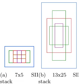
Figure 4.5 Stack layout for 7x5 and 13x25 filter sizes . . . 49
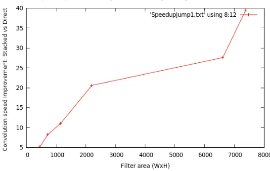
Figure 4.8 Speed Improvement using the Stacked Integral Image vs. Kernel Integral
Image and Direct Convolution Scene=400x300, Model=55x115 . . . 52
Figure 4.9 Speed Improvement using the Stacked Integral Image vs. Kernel Integral Image and Direct Convolution Scene=400x300, Model=13x25 . . . 52
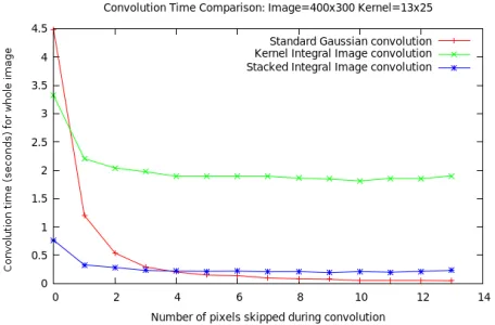
Figure 4.10 Image and Direct convolution . . . 53
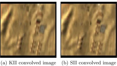
Figure 4.11 KII convolution and SII convolution . . . 53
Figure 4.12 KII and SII convolution difference images (increased 10 times) w.r.t. Direct method . . . 54
Figure 5.1 Mean shift defines a path to a local density maximum [10] . . . 56
Figure 5.2 Principle of Unscented Transform [11] . . . 64
Figure 6.1 Result of Birchfield’s Elliptical Tracker [12] . . . 75
Figure 6.2 Image; Segmentation result; Blob output; Morphological grow [13] . . . . 77
Figure 6.3 Low SVM margin; High SVM margin [14] . . . 78
Figure 6.4 Dashed rectangle=Initial location. Solid rectangle=Final location; Graph of corresponding SVM scores [14] . . . 80
Figure 6.5 B-spline curve and curve normals along which high contrast features are sought; Evolution of multimodal state density [15] . . . 81
Figure 6.6 Icondensation with Importance sampling and reinitialization [16] . . . 83
Figure 6.7 Icondenstaion tracking in high speed motion [16] . . . 84
Figure 6.8 Tracking using Meer’s mean shift [17] . . . 86
Figure 6.9 Number of iterations (Left) and SSD (Right) w.r.t. frame index [18] . . . 88
Figure 6.10 Yang’s method (Top) vs. color histogram only (Bottom) [1] . . . 90
Figure 6.11 Tracking time vs. (Left) frame index and (Right) number of particles [1] 90 Figure 6.12 MTT system; Track gates [19] . . . 91
Figure 6.13 Original components; Gaussian Sum approximation; Piecewise Gaussian approximation [20] . . . 96
Figure 6.14 Original image sequence; Single mode tracking [20] . . . 97
Figure 6.15 Multiple hypothesis; Multi hypothesis tracking [20] . . . 98
Figure 6.16 (a-b-e) Intersection surfaces (S1, S2, S); (c-d) Difference between the surfacesS1 andS2 extracted from two dynamical models; (f) Intersection surfaces when two predictions at instantt,A1andA2are equidistant from yj. [21] . . . 99
Figure 6.17 Ant sequence. (a) Frames at t-2, t-1, t, t+1; (b) Tracking result obtained with EPF; (c) Regression Error Characteristic (REC) curves. [21] . . . 100
Figure 6.18 Rao-Blackwellized: Sine wave tracking [22] . . . 101
Figure 6.19 Interacting targets are not independent; Target with best likelihood hi-jacks nearby target filters [23] . . . 101
Figure 6.20 MRF based MCMC sampler performance comparison [23] . . . 103
Figure 6.21 MRF based MCMC sampler algorithm [23] . . . 103
Figure 7.1 Blender test environment. Tank with red boundary is the target. . . 106
Figure 7.3 SKS and PF tracking with Bounding Box . . . 111
Figure 7.4 SKS and PF tracking with Complete Occlusion for 5 frames . . . 111
Figure 7.5 SKS and PF tracking with vertical and horizontal movements . . . 112
Figure 8.1 Change in size of target at different elevations produces different number of feature points. . . 114
Figure 8.2 Minimum target size in pixels, to achieve correct detection via SKS . . . 114
Figure 8.3 Change in gradient directions when shadow is cast. . . 115
Figure 8.4 Overall Proposed System. . . 119
Figure 9.1 Interaction: Best likelihood target hijacks nearby target filters [23] . . . . 125
Figure 9.2 TC1: Regular Sampling: Particle swap . . . 133
Figure 9.3 TC2: Regular Sampling: Particle hijack . . . 133
Figure 9.4 TC3: Charged Sampling: Particle hijack prevented . . . 134
Figure 9.5 TC4: Charged Sampling: Particle hijack prevented (low variance) . . . . 135
Figure 9.6 TC5: Charged Sampling: Occlusion handled: No Particle hijack . . . 135
Figure 9.7 Plot of rejection count with Probabilistic Charged Resampling . . . 136
Figure 10.1 Combined PRCA and SKS detection with Charged Resampling during target cross over and changing scene elevation, with low particle variance 141 Figure 10.2 Combined PRCA and SKS detection with Charged Resampling during target cross over and changing scene elevation, with high particle variance 141 Figure 10.3 Combined PRCA and SKS detection with Charged Resampling to pre-vent particle hijack during target interaction frames, and changing scene elevation, with high particle variance . . . 142
Figure 11.1 SKS and PF Hierarchical tracking: Single Target . . . 146
Figure 11.2 SKS and PF Non-Hierarchical multiple target tracking . . . 147
Figure 11.3 SKS and PF Hierarchical multiple target tracking . . . 147
Figure 11.4 SKS and PF Hierarchical multiple target tracking . . . 148
Figure 11.5 SKS and PF Hierarchical multiple target tracking . . . 149
Figure 11.6 Data Association accuracy for the Target Crossover test case . . . 150
Figure 11.7 Data Association accuracy for no Target Crossover test case . . . 151
Figure A.1 Operation for (a) B-MAC, (b) A-MAC-UR and (c) A-MAC-HS: Sender (A), intended (B) and unintended (C, D and E) receivers . . . 164
Figure A.2 Power consumption for B-MAC, A-MAC-UR and A-MAC-HS for the five considered scenarios as a function of the check interval T i . . . 176
Figure A.3 Finite-state machines for (a) B-MAC, (b) A-MAC-UR and (c) A-MAC-HS.178 Figure A.4 Throughput of A-MAC-HS and B-MAC as a function of the offered load. 178 Figure B.1 Munsell Color Model (source: wikipedia). . . 187
Figure B.3 Left: The interpreted color image (flatColorImage). Right: The image (recoloredImage) with the grey level bins reclassified as White or Black colors. Notice that not all white pixels from the image on the left, remain as white in the recolored image on the right. This is achieved by using
the histogram to calculate new threshold for white. . . 189
Figure B.4 Left: The recolored image (recoloredImage). Right: Edges for lane mark-ings (skeletonImage) as single pixels without the need for thinning the edges and without converting two edges of a lane to a single edge. . . 190
Figure B.5 Left: The edges for lane markings (skeletonImage) as single pixels. Cen-ter: Hough lines (houghImage). Right: Minimized set of Hough line segments (LineSegments). . . 191
Figure B.6 Straight road with two lane markings. . . 192
Figure B.7 Straight road with lane markings and pedestrian crossing. . . 193
Figure B.8 Curved road. . . 193
Figure B.9 Arbitrary road markings. . . 194
Figure B.10 Low light lane detection. . . 194
Figure C.1 A set of 7 cameras defining a convex polygon. Cameraiis denoted ci, and has angular field of view of θi. . . 198
Figure C.2 Zoom-out: the focal length is shortened from f0 to f, moving the focal plane closer to the focal point. Before the zoom, the length of the focal plane was 2xo, subtending an angle of 2θ0 (only half of the focal plane is shown in this right triangle). After the zoom, the same portion of the visual field only occupies a length of xon the focal plane. So the camera can see more, but a given object occupies fewer pixels on the focal plane. 200 Figure C.3 Zoom-in: the focal length is lengthened from f0 tof, moving the focal plane farther from the focal point. The length of the physical focal plane is 2xo, subtending an angle of (2θ0). (Typically, 2θ0 might be 35mm.) Before the zoom, if we were to image a point at distance f, we would see an additional width of dx. However, when we zoom, and actually move the focal plane to f, we only image a range ofx0, a reduction in the field of view. . . 201
Figure C.4 Three points on the contour of a formation. To maintain convexity, the center point must not align with the line between its two neighbors. . . . 204
Figure C.5 The magnitude of the control applied to a typical robot in a ring as a function of the radius of the ring. We observe that the equilibrium state for this rings occurs at r= 3.3. . . 205
Figure C.6 The single merged 360◦ panoramic image. . . 206
Figure C.7 Sample pre-computed cropped images. . . 206
Chapter 1
Introduction
1.1
Object Tracking
Object tracking is the task of detecting and following an object of interest, over a period of time. A vision based tracking system detects and tracks objects in a sequence of images. Unlike sensors such radar and lidar, which emit energy to detect objects, vision-based systems are passive because they only receive signals. This thesis focusses on vision-based tracking systems.
Object tracking is an important task in a variety of applications such as people tracking, vehicle tracking, animal tracking etc. Tracking people at national boundaries is done for se-curity reasons. People tracking is also done for surveillance at locations such as airports, rail terminals, landmarks, buildings, homes etc. The transport department tracks people to control traffic signals, estimate road utilization, plan for growth etc. Vehicle tracking is used in traffic monitoring, delay estimation, reroute planning etc. Tracking vehicles is of prime importance when designing autonomous vehicles. One of the key test in the Grand Challenge conducted by DARPA in 2007, was to test autonomous vehicle behaviour in multiple situations such as stop sign priority following, right of away decision making, suitable lane merging etc. Animal tracking is used for monitoring their behaviour and to gather statistics. It is helpful to study migration patters, reproductive cycles, population estimation etc. Tracking of blood clots, or-gans etc. is important in medical applications and robotic surgery. Hence, object tracking is the center piece in a variety of applications.
Object tracking can be categorized as single object tracking and multiple object tracking
more than one target is called “Multiple Target Tracking” (MTT) in literature, while that for a single object is called “Object Tracking” or “Target Tracking”.
1.2
Problem Description
While object tracking seems to be a natural extension of object detection algorithm, it has its own set of difficulties. Detection algorithms focus on how well to describe the object (model) so that they can be reliably detected in the scene (image). Hence, detection algorithms provide a good object detection and matching technique, but have to handle problems such as image noise, object rotation and scale changes, partial occlusion, low resolution etc. In addition to these problems, tracking algorithms have to further handle problems such as complete object occlusion, continuous scale change and rotation, multiple detector inputs, simultaneous target and scene movement etc. Hence, designing a robust tracking algorithm is not easy and does not have a “one size fit all” approach. All the above problems get even further compounded when the system is designed to track not one, but multiple objects. Hence, multiple object tracking systems have to handle problems such as correct continuous association of observations with targets (data association problem), maintaining correct separation of all target track estimates when multiple targets come close to each other (data merge problem), varying and different dynamics of each target, scene dynamics, varying resolution etc. Hence, designing a multiple object tracking system is an even more challenging task.
This thesis describes a solution to track multiple objects at varying resolution levels in a dynamic scene environment. Thus, it handles the problems of data association, data merge, low resolution, occlusion, rotation/scale changes, changing object dynamics and scene movement.
1.3
Tracking system compnents
The principle of object tracking is to determine what part of the image best corresponds to the reference model of one or more objects and then to keep tracking it in successive image frames. Hence the key elements of a tracker system are an “object descriptor/detector” and an “object tracker”. The descriptor algorithms can be broadly classified as either “deterministic” or “density” methods. The tracker algorithms can be broadly classified as either “deterministic” and “stochastic” methods.
The density descriptor methods are more robust to partial occlusions etc. Examples of such descriptors are color histograms, etc.
The deterministic tracker methods assume that the object to be tracked is present in the image, in some local neighborhood, and they attempt to find the object. Examples of such tracking methods are “mean shift” algorithm etc. These algorithms assume the search is de-terministic and hence can fail in case of total occlusion, presence of other objects with similar descriptor, or large object displacements etc.
Stochastic tracker methods are more robust to total occlusion by describing the object location probabilistically. Examples of such tracking methods include “Kalman filter”, “Particle filter” and variations.
1.4
This Thesis
This thesis provides a novel multiple object tracking system in a dynamic scene environment, using vision-based algorithms. It provides innovations in areas of both object detection and object tracking and hence covers background and novelty in both these areas. The layout of the thesis is shown below:
• Chapter 1: Introduction
• Chapter 2: Geometric Descriptor Algorithm
This chapter covers the geometric descriptor algorithm literature, followed by the final choice of a geometric desciptor algorithm, Simple K Space (SKS), in the proposed tracking system.
• Chapter 3: Radiometric Descriptor Algorithm
This chapter summarizes radiometric descriptor algorithms, and then proposes a novel ra-diometric algorithm, “Pattern Recognition by Cluster Accumulation” (PRCA), to detect objects at low resolution while being rotation invariant.
• Chapter 4: Convolution Algorithm
This chapter describes a novel convolution algorithm, “Stacked Integral Image”, which provides a significant speed-up, when performing non-uniform filtering (such as Gaussian kernel).
• Chapter 5: Review of Tracking Algorithms
• Chapter 6: Review of Visual Detection and Tracking Systems
This chapter is a literature survey of detection and tracking systems, which covers some of the prominent combination of detection and tracking algorithms. The problem of particle hijack (data merge) is highlighted for later reference.
• Chapter 7: Initial Detection and Tracking System
This chapter describes an initial design of the detection and tracking system, along with initial test results.
• Chapter 8: Initial System Problem Resolution and Extension
This chapter describes the problems observed with the initial tracking system and the proposed novel solutions. Specifically, the problem of detection at low resolution as seen in the initial system design, and the problem of particle hijack (data merge) as seen in detection and tracking systems suvey, are emphasized. Additionally, the proposed novel extension, to handle the scene movement dynamics, “Hierarchical Particle Filter”, is introduced. The chapter summarizes with the proposed complete system.
• Chapter 9: Particle Hijack and Charged Resampling
This chapter solves the particle hijack (data merge) problem with a novel “Charge Re-sampling” method. It describes the proposed algorithm along with demonstration of algorithm capabilities.
• Chapter 10: Multiple Object Tracking with Multiple Detectors
This chapter describes how the multiple object tracking system, with radiometric detector input from PRCA, and geometric detector input from SKS, handles the data association problem, along with Charge Resampling algorithm to prevent particle hijack. It demon-strates the system capabilites with these novelties.
• Chapter 11: Hierarchical Multiple Object Tracking System
Finally, the complete system is presented in this chapter, which adds the Hierarchical Particle Filter design, to the multiple object tracking system from the previous chapter, in order to handle scene dynamics. It demonstrates the capability of the hierarchical design to handle scene dynamics, along with performance statistics of such a system in various particle count and variance settings.
• Chapter 12: Novel Contributions
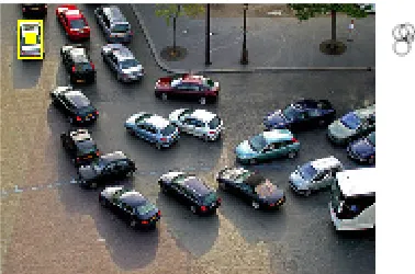
A recent article in the October, 2010 issue of the IEEE Spectrum magazine, highlights the importance of object tracking and the main challenges therein, in the context of surveillance video as captured by a UAV. The image capture of the article is shown in figure 1.1, which highlights some of the notorious challenges in object surveillance.
1. The text highlighted in the blue rectangle mentions “tracking big swarms of objects”, which is the same problem as, and shows the importance of, multiple object tracking.
2. The text highlighted in the yellow rectangle mentions “cars are exceedingly small (usually no more than 30 pixels)”, which is the same problem as detection at low resolution, for which the novel PRCA algorithm has been proposed.
3. The text highlighted in the brown rectangle mentions “two vehicles wont choose a collision course”, which is the same as interacting targets and the particle hijack problem, for which the novel Charge Resampling algorithm has been proposed.
4. The text highlighted in the pink rectangle mentions “noisy optical flow ... lots of motion”, which is the same as simultaneous scene and target movement problem, for which the novel Hierarchical Particle Filter design has been proposed.
1.5
Grants
This work was partly supported by AFOSR under grant no. FA9550-07-1-0176 and ARO under grant no. W911NF-05-1-0330.
1.6
Appendices
1.6.1 Written Qualifier Exam
1.6.2 DARPA Urban Challenge
While doing formal research in computer vision, the author also volunteered time to provide complete vision solution to the NCSU sponsored team “Lone Wolf”, which took part in the DARPA Urban Challenge in 2007. As part of this work, a lane detection system was developed using computer vision techniques to guide the autonomous vehicle within lane boundaries. This result was published in SPIE [24] and the paper content is provided in Appendix B.
1.6.3 Robot Control
Chapter 2
Geometric Descriptor Algorithm
The purpose of adescriptoris to able to describe a target in such a way such that it can be easily
detected within a scene. When the descriptor utilizes the geometric properties of an object such as corners and edges, then it is known as ageometric descriptor. These descriptors perform well when the size of the target in the image is big enough to measure these geometric properties and the signal has not been heavily distorted by blur or noise. The following sections briefly describe some of the existing geometric descriptor algorithms and the final choice of geometric descriptor that is used in our tracking system.
2.1
Edge Oriented Histogram
In [1], Yang et al. build an edge oriented histogram to get the benefits of contour based detectors. To detect edges, the color image is first converted to grayscale intensity image and edges are detected using horizontal and vertical Sobel operators Kx and Ky.
Gx(x, y) =Kx∗I(x, y) (2.1)
Gy(x, y) =Ky∗I(x, y) (2.2)
S(x, y) =
q
G2
x(x, y) +G2y(x, y) (2.3)
θ=arctan(Gy(x, y)/Gx(x, y)) (2.4) A thresholdT is applied to the edge strengthS(x,y) and the edges are counted intoK bins based on their angle θ with their strengths S(x,y). The edge oriented histogram for a sample image is shown in figure 2.1 [1].
Figure 2.1: Image; Edge Image; Edge Oriented Histogram [1]
to clutter and may be more time-consuming than color histograms. Hence Yang et al. [1] use a combination of color information and the edge oriented histogram to improve performance.
2.2
Lowe’s Scale Invariant Feature Transform
David Lowe introduced theScale Invariant Feature Transform(or SIFT) [25] algorithm to detect and describe local features in images. The SIFT features are local and based on the appearance of the object at particular interest points, and are invariant to image scale and rotation. They are also robust to changes in illumination, noise, and minor changes in viewpoint. They are highly distinctive and allow for correct object identification. SIFT is described in detail here as it bears some similarity to our SKS feature descriptor, which will be described in section 2.5.
2.2.1 Scale space extrema
At this stage the interest points, called keypoints in the SIFT framework, are detected. For this, the image is convolved with Gaussian filters at different scales, and then the difference of successive Gaussian blurred images are taken. Keypoints are then taken as maxima/minima of the Difference of Gaussian (DoG) that occur at multiple scales. Specifically, a DoG image D(x, y, σ) is given by:
where L(x, y, kσ) is the convolution of the original image I(x, y) with the Gaussian blur G(x, y, kσ) at scalekσ, i.e.,
L(x, y, kσ) =G(x, y, kσ)∗I(x, y) (2.6) The convolved images are grouped by octave (an octave corresponds to doubling the value ofσ). Keypoints are identified as local minima/maxima of the DoG images across scales. This is done by comparing each pixel in the DoG images to its eight neighbors at the same scale and nine corresponding neighboring pixels in each of the neighboring scales. If the pixel value is the maximum or minimum among all compared pixels, it is selected as a candidate keypoint. This scale space extrema method is similar to that developed by [26]. The difference of Gaussian operator can be seen as an approximation to the Laplacian used there. The figure 2.2 shows Difference of Gaussian and scale space extrema detection.
Figure 2.2: Gaussian of Image; Difference of Gaussian of Image; Scale Space Extrema [2]
2.2.2 Keypoint localization
D(x, y, σ) with the candidate keypoint as the origin [2].
2.2.3 Orientation assignment
Each keypoint is assigned one or more orientations based on local image gradient directions. This achieves invariance to rotation as the keypoint descriptor can be represented relative to this orientation and therefore achieve invariance to image rotation. First, the Gaussian-smoothed image L(x, y, σ) at the keypoint’s scale σ is taken so that all computations are performed in a scale-invariant manner. For an image sample L(x, y) at scale σ, the gradient magnitude, m(x, y), and orientation,θ(x, y), are precomputed using pixel differences:
m(x, y) =
q
(L(x+ 1, y)−L(x−1, y))2+ (L(x, y+ 1)−L(x, y−1))2 (2.7)
θ(x, y) = tan−1
L(x, y+ 1)−L(x, y−1) L(x+ 1, y)−L(x−1, y)
(2.8)
The magnitude and direction calculations for the gradient are done for every pixel in a neigh-boring region around the keypoint in the Gaussian-blurred imageL. An orientation histogram with 36 bins is formed, with each bin covering 10 degrees. Each sample in the neighboring window added to a histogram bin is weighted by its gradient magnitude and by a Gaussian-weighted circular window with aσ that is 1.5 times that of the scale of the keypoint. The peaks in this histogram correspond to dominant orientations.
2.2.4 Keypoint descriptor
The contribution of each pixel is weighted by the gradient magnitude, and by a Gaussian with σ 1.5 times the scale of the keypoint. Histograms contain 8 bins each, and each descriptor contains a 4×4 array of 16 histograms around the keypoint. This leads to a SIFT feature vector with (4×4×8 = 128elements), as shown in figure 2.3.
Once the descriptor has been built, object recognition is done via SIFT features, as shown in figure 2.4.
2.3
Mikolajczyk’s Harris Laplace detector
In [3], Mikolajczyk and Schmid use the scale space concept of [26] to compare four interest point detectors:
Figure 2.3: Image Gradients; Keypoint descriptor [2]
Laplacian :|s2(Lxx(x, s) +Lyy(x, s))| (2.10)
Difference of Gaussian :|I(x)∗G(sn−1)−I(x)∗G(sn)| (2.11)
Harris function : det(C)−αtrace2(C) (2.12) where,
C(x, s,˜s) =s2∗G(x,s)˜ ∗
"
L2x(x, s) LxLy(x, s) LxLy(x, s) L2y(x, s)
#
(2.13)
The scalesis called the derivative scale, and the scale ˜sis called the integration scale. The comparison of using the four methods above to detect points at characteristic scale is given in figure 2.5, which shows the Laplacian as the best performer.
Figure 2.5: Percentage of correct points detected [3]
To further improve the performance, they suggest using two functions to detect the scale invariant points. They use the Harris function (2.12) to localize points in 2D and then select points for which the Laplacian attains a maximum over scales. They refer to it as the Harris-Laplacian detector and the resulting detection performance is indicated in figure 2.6. The authors further extended the interest point detector to be affine invariant in [27] and [28]. We use the Harris-Laplace style detector in SKS 2.5.
2.4
Dalal’s Histogram of Oriented Gradients
Figure 2.6: Performance of Harris Laplace detector [3]
orientation in localized portions of an image. This method is similar to that of edge orientation histograms, scale-invariant feature transform descriptors and shape contexts, but differs in that it computes on a dense grid of uniformly spaced cells and uses overlapping local contrast normalization for improved performance. The paper [4] uses these HOG descriptors to detect humans in an image.
The method is based on evaluating well-normalized local histograms of image gradient orientations in a dense grid. The basic idea is that local object appearance and shape can often be characterized rather well by the distribution of local intensity gradients or edge directions, even without precise knowledge of the corresponding gradient or edge positions. In practice this is implemented by dividing the image window into small spatial regions (“cells”), and for each cell, accumulating a local 1-D histogram of gradient directions or edge orientations over the pixels of the cell. The combined histogram entries form the representation. For better invariance to illumination, shadowing, etc., it is also useful to contrast-normalize the local responses before using them. This can be done by accumulating a measure of local histogram “energy” over somewhat larger spatial regions (“blocks”) and using the results to normalize all of the cells in the block. These normalized descriptor blocks are called Histogram of Oriented Gradient (HOG) descriptors. Tiling the detection window with a dense (overlapping) grid of HOG descriptors and using the combined feature vector in a conventional SVM based window classifier provides a detection chain.
because the subsequent descriptor normalization achieved similar results. RGB and LAB color spaces give comparable results, but restricting to grayscale reduces performance.
Gradients were computed using Gaussian smoothing followed by one of several discrete derivative masks. Simple 1-D [1,0,1] masks at σ = 0 worked best. Using larger masks de-creased performance, and smoothing damaged it significantly. For color images, gradients were calculated for each color channel and the one with the largest norm was taken as the pixels gradient vector.
Each pixel calculates a weighted vote for an edge orientation histogram channel based on the orientation of the gradient element centered on it, and the votes are accumulated into orientation bins over local spatial regions called “cells” (rectangular or radial). The orientation bins are evenly spaced over 0◦−180◦ (“unsigned” gradient”) or 0◦−360◦ (“signed” gradient”). To reduce aliasing, votes are interpolated bilinearly between the neighboring bin centers in both orientation and position. The vote is a function of the gradient magnitude at the pixel. Using the magnitude itself gives the best results. Taking the square root reduces performance slightly. Fine orientation coding gave good performance, whereas spatial binning can be rather coarse. Increasing the number of orientation bins improves performance significantly up to about 9 bins (unsigned), but makes little difference beyond this. Including signed gradients decreases the performance.
Effective local contrast normalization is required since gradient strengths vary over a wide range owing to local variations in illumination and foreground-background contrast. Cells are grouped into larger spatial blocks and contrast normalized at block level. The final descriptor is the vector of all components of the normalized cell responses from all of the blocks in the de-tection window. Blocks overlap so that each scalar cell response contributes several components to the final descriptor vector, each normalized with respect to a different block.
Denote v to be the unnormalized descriptor vector,kvkk be its k-norm for k= 1,2, and be a small constant. Block Normalization is done using L2-Hys: L2-norm followed by clipping (limiting the maximum values ofv to 0.2) and renormalizing.
The final environment uses: RGB color space with no gamma correction; [1,0,1] gradient filter with no smoothing; linear gradient voting into 9 orientation bins in 0◦−180◦; 16×16 pixel
Figure 2.7: Gradient Image; Positive SVM weights; Negative SVM weights; Image; HoG descriptor; Positive weighted descriptor; Negative weighted descriptor [4]
2.5
Simple K Space
In [5, 6, 7, 8], Krish et al. proposed an accumulative framework for reliably detecting target objects across scale and orientations, in cluttered environments with occlusions.
The framework, called the Simple K-Space (SKS) algorithm, uses an accumulative approach reminiscent of the well known Generalized Hough Transform introduced by Ballard [30] to recog-nize general shapes. Accumulator-based methods are highly parallel and use simple arithmetic. Noise and isotropic distortions tend to average out. The algorithm is invariant to translation, rotation, scale (zoom) and robust to illumination changes, background clutter and occlusion as well as view point changes.
The salient points of a target image are extracted using the scale invariant keypoints of a Harris-Laplace detector. A descriptorθis built around eachsalient point using the distribution of gradients around that point, for a scale normalized radius and a fixed set of angular bins. The location of the point is characterized by (r,θ), which represent the distance to a reference point and the descriptor at that point, respectively.
A target object model ψ :Rd+1 → [0,1] is defined with respect to the reference point such
that ψm(r,θ) gives the confidence that descriptor θ occurs in the mth model at a distance r from the reference point Cm. Given a collection of M models, {ψ1, ψ2,· · ·, ψM}, the goal is to determine if there are instances of a particular model in an image I, by searching for all instances of areference point in the observed image.
Am(x) = J
X
j=1
ψm(rj,θj) (2.14)
This is like normalizing the feature vector for translation, rotation, scale etc. It accumulates the confidence that a candidate reference point point xdescribes the instance of the model m in the imageI. Since ψm is precomputed (from the target model), the calculation simplifies to J lookups. The best matching model, ˆψ, is given by the model function which gives the highest peak value in the accumulator:
ˆ
ψ= arg max
m,x Am(x) (2.15)
Hence, the goal is to look for that combination of target model m and reference point x, which gives the maximum accumulator score.
Although the descriptor θ mentioned above talks about using the Harris-Laplace interest points, but other different descriptors can be used for different situations, while keeping the model matching philosophy the same. The figure 2.8 shows the accumulator array (a two dimensional accumulator in this case) for a good match and a bad match. The image on the left shows a tank silhouette matched with a tank model of the rotated and scaled version of itself which results in a sharp peak. The image on the right shows the same tank silhouette matched with the model of a different tank resulting in no well defined peak.
2.6
Geometric Descriptor Choice
Chapter 3
Radiometric Descriptor Algorithm
A simple size-based target classification would give three categories of targets in a scene image. The “very small” targets (e.g. sub-pixel), which have only radiometric signature that can be used for comparison. The “large” (resolved) targets, which have sufficient gradient information that can be used to detect them. The “small” (partially resolved) targets, where the gradient information can be computed but is not always accurate. This chapter deals with the “small” sized targets.
As mentioned in the previous chapter, geometric descriptors perform well when the target size is reasonably big enough to extract the relevant geometric features such as corners and edges. When the target size is small or when the image signal is noisy such that the corners and/or edges cannot be reliably detected, then relying on geometric descriptors is not sufficient. The Johnson criteria [31] suggests that even for a human observer, identifying a target requires significantly higher resolution than merely detecting it. Hence, for “small” or “blurred” targets, radiometric features can give better results and getting the target’s radiometric properties as a descriptor would perform better. Such descriptors are called radiometric descriptors and they can detect objects reliably in noisy environments. The following sections briefly discuss some of the existing radiometric descriptor algorithms, followed by a new radiometric descriptor algorithm (PRCA), and the final choice of radiometric descriptor algorithm to be used in our tracking system.
3.1
Color Histograms
In this algorithm, the feature descriptor at a point is a histogram of color values in the neigh-borhood of the given point.
at 0, a function b : R2 → {1 . . . m} maps pixel at location {xi} to the index b(xi) of the histogram bin corresponding to the color of that pixel. Overlap of color histograms can then be computed between model and target [32]. Hence the color histogram is a distribution of colors around a point, expressed as a histogram and written as h(I) = P
i∈I
b(xi). Such a color histogram is used as a feature descriptor in [33].
Although a color histogram is robust against noise and partial occlusion, it suffers from illumination changes, or the presence of confusing colors in the background and ignores spatial layout information.
3.2
Viola’s Rectangles
In [9] Viola and Jones have suggested a simple form of Haar like features in the form of rect-angles. These rectangle features can be in the form of 2-rectangle, 3-rectangle or 4-rectangle features, as shown in figure 3.1 [9]. Each rectangle feature computes the sum of pixel values which lie within the white rectangle area from the sum of pixel values in the grey rectangle area.
Figure 3.1: Two (A,B), Three (C) and Four (D) rectangle features. [9]
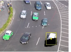
In order to compute the value of the rectangle feature very rapidly, they introduce the idea of an intermediate representation for the image called the “Integral Image”. The integral image at locationx,y contains the sum of pixels above and to the left ofx,y, inclusive:
ii(x, y) = X x0≤x,y0≤y
i(x0, y0) (3.1)
quickly computed using the following recurrences:
s(x, y) =s(x, y−1) +i(x, y) (3.2) ii(x, y) =ii(x−1, y) +s(x, y) (3.3) Using the integral image any rectangular sum can be computed in four array references, as shown in figure 3.2 [9].
Integral Image Sum of pixels in rectangle
Figure 3.2: Left: Integral Image. Right: The sum of pixels in a rectangle. [9]
The Integral Image at a point (x, y) is the sum of pixels above and left of it, including itself. The sum of the pixels within rectangle D can be computed with four array references. The value of the integral image at location 1 is the sum of the pixels in rectangle A. The value at location 2 is A + B, at location 3 is A + C, and at location 4 is A + B + C + D. The sum within D can be computed as 4 + 1−(2 + 3). Hence, computing sum of pixels within a rectangular area can be computed very quickly. Eventually, these rectangles are used as feature descriptor for regions of interest. Changing the size of the rectangles adapts them to scale.
3.3
New Radiometric Descriptor Developed: PRCA
is a cluster based rotation invariant radiometric algorithm. The following sections introduce and describe the PRCA algorithm, followed by experimental results of PRCA and the resulting conclusion.
3.3.1 PRCA Overview
In PRCA, clustering provides dimension reduction by choosing the representation of given data which requires the fewest clusters to characterize it. Other techniques, such as PCA [35], use eigen decomposition for dimension reduction. The popular K-means [35] clustering algorithm works well when the number of clusters k is known. When k is not known, it can be estimated with iterative methods, such as ISODATA [36]. In contrast, “density based clustering” algorithms, such as DBSCAN [37], do not require the number of clusters, but do require other parameters such as densityd, to generate “connected components” style “clusters” that we use here. In [38] Nanni et al. addressed the difficulty of finding good features for every pattern in a class, which led them to propose a cluster-based pattern discrimination (CPD) technique. It assigns a test pattern to the class with the highest classifier score, which it has computed by partitioning the classes into clusters, defining a subspace for each cluster, and testing similarity by a classifier. By dividing a class into clusters, they could find features specific to some subset of patterns in each of the classes that effectively distinguished the classes from each other, even though none of the features were well suited to the entire set of patterns. In this paper we propose a cluster based pattern recognition method that exploits those clusters themselves as features by searching for such clusters in test images without relying on geometric features (like corners or edges) of the target. We manage the undesirable sensitivity of clustering to illumination or perspective with an accumulator based technique. The following section describes this PRCA algorithm in detail.
3.3.2 PRCA Approach
Consider an image as a rectangular array ofR, G, B pixels. Given a model imageIm, the goal is to detect it in another (scene) image Is. To achieve this, we generate clustered images Cm and Cs, for the model and scene images Im and Is respectively, and then use an accumulator to robustly match clusters inCm with clusters in Cs.
clusters in the two images. Further, in PRCA, the accumulator approach provides invariance to translation, rotation and robustness against occlusion, distortion and illumination changes. The next section explains clustering in the algorithm.
Clustering
Any connected component style algorithm can be used to do clustering. We propose to use a modification of the density based clustering algorithm DBSCAN [37]. This algorithm needs density parameter,ρ, but does not need the number of clusters parameterk.
Using DBSCAN algorithm directly in an R, G, B image would involve building a five di-mensional search space: x, y, R, G, B, and then forming clusters by searching in the 5-D space for regions with point density greater than ρ.
To reduce this computation and search complexity, the algorithm is modified to take an additional similarity threshold parameter, γ, so that clustering is done in two dimensional space x, y. Clusters are formed if the (R, G, B) difference of neighboring pixels is less than γ and the point density of such R, G, B similar pixels at neighborhood of every point in the cluster, is greater than ρ. As explained in equation 3.4, pixel (xi, yi) is added to cluster Cn, which already has (xk, yk) as its member, if the similarity and density constraints are met.
N eigh(xi, yi) ={(xj, yj)|(xj, yj)∈8 connected(xi, yi)} Sim(xi, yi) ={(xj, yj)|(xj, yj)∈N eigh(xi, yi)∧ k(Ri, Gi, Bi)−(Rj, Gj, Bj)k2 < γ} Cn(xk, yk) ={(xi, yi)|Sim(xi, yi)/N eigh(xi, yi)> ρ∧(xi, yi)∈N eigh(xk, yk)}
(3.4)
Hence a single cluster in an image is a connected set of pixels whose (R, G, B) difference is within the threshold γ and every point in such a cluster has a density greater than ρ. A clustered image is then the image where such cluster of pixels have been formed. The details of the algorithm can be viewed in [37].
Given a model image (target chip) Im, the modified DBSCAN algorithm generates a clus-tered imageCm, withNm number of clusters, as shown in figure 3.3a. SimilarlyNsclusters are formed in the clustered image Cs from the scene Is, as shown in figure 3.4. The Cm clusters now act as features that are to be detected in the set of Cs.
(a) Model & Cluster 1 (b) Model & Cluster 2
Figure 3.3: Model Image Im and its Clustered image Cm
Figure 3.4: Scene ImageIs1 and its Clustered image Cs1
Cluster Match
Thekthpixelpkis denoted by a triple of colorspk= (rk, gk, bk), where each color is normalized, e.g. rk = Rk/kRk, Gk, Bkk. A cluster therefore is a set of such pixels Γi = {pi1, pi2, ..pin}. However, rather than representing this set by its membership, we use its statistics Xi = [< r >Γi, < g >Γi, < b >Γi, ωi] where < . > denotes the sample mean and ωi is the cardinality of
Γi. Thus to compareXmi , theith cluster inCm, with Xsj, thejthcluster inCs, we calculate the match score η, using L2 norm k.k2, as shown in equation 3.5.
ωbig = max(ωi, ωj) ωi =ωi/ωbig ωj =ωj/ωbig η(Cmi , Csj) =X¯mi −X¯sj
2
(3.5)
The score η(Cmi , Csj) must be above a threshold λto be a valid match. The values ωi and ωj are normalized by the bigger of those two numbers, before calculating the norm, as shown in equation (3.5).
Hence, for each model clusterCmi , this step finds the best matching scene clusterCsj, in terms of color similarity and number of pixels (size of cluster). Since the match score is computed for every pair Ci
m : i= 1..Nm and Csj :j = 1..Ns, in Cm and Cs respectively, a list of match score, Lim, is kept for every model cluster, i.e. for a given model cluster, there is a ranked list of matching scene clusters, based on their match score.
Lmi ={. . . , Csp, Csq, . . .|η(Cmi , Csp)> η(Cmi , Csq),
η(Cmi , Csr)> λ,∀r} (3.6)
Hence, this matching process produces a ranked list of scene clusters, for every cluster in model image, as shown in figure 3.7a. It is very likely that a given model cluster has split into two or more clusters in the scene, or two or more model clusters have merged as a single cluster in the scene, and this impacts the match score of equation (3.5). Splitting is merging is handled in the accumulator, as explained in the next section.
Pair wise match potential
with therth cluster inCs, then, the confidence in this pair of matches is high if the proportion of pixels along the path fromithcluster to theqthcluster inCm, that are neither in clusterior q, must be similar to the proportion of pixels along the path from jth cluster to the rth cluster inCs, that are neither in clusterj nor in cluster r. This notion of pair wise cluster similarity is termed asWalk Ratio, as shown in figure 3.6.
Figure 3.6: Walk ratio of clusters in model (Mi,Mj) and scene (Sv,Sw) image are close for a good match
The corresponding Walk Ratio Error (W RE) is calculated using image pixels pk and set cardinality |.|as follows:
W Rn(Cmi , Cmq) =
{pk|pk∈/ Cmi ∧pk∈/Cmq} /
{pt|pt∈Cmi ∨pt∈Cmq}
W Rd(Cmi , Csj, Cmq, Csr) = abs(W Rn(Cmi , Cmq)−W Rn(Csj, Csr)) W Rm(Cmi , Csj, Cmq, Csr) = max(W Rn(Cmi , Cmq), W Rn(Csj, Csr)) W RE(Cmi , Csj, Cmq, Csr) =W Rd(Cmi , Csj, Cmq, Csr)/W Rm(Cmi , Csj, Cmq, Csr)
(3.7)
For a given choice of the triple Cmi , Csj, Cmq, the rth cluster Csr which gives the minimum Walk
Ratio Error (W RE(Cmi , Csj, Cmq, Csr)) is chosen, and that error is added to Pair Error Sum P ES(Cmi , Csj), as follows:
M W RE(Cmi , Csj, Cmq) = min
r (W RE(C i
m, Csj, Cmq, Csr)) P ES(Cmi , Csj) =X
q
(M W RE(Cmi , Csj, Cmq)) (3.8)
model clusters. This gives a notion of pair wise potential to the simple match score that was computed in the previous section. ThePair Error SumP ES(Cmi , Csj) is normalized to lie in the range 0. . .1 and is added to the original match error to get a total error value which represents not only how good a model cluster matches with a scene cluster, but also how compatible this matching pair is with respect to all other matching pairs.
Accumulator
Recall that a model contains a single target, which may consist of several clusters. For every model cluster Cmi : i = 1..Nm, a distance from the center of the cluster to the center of the model image is computed and stored. For the ith model cluster Cmi , we call this distance Dmi . Thus the center of the model image is the reference point and the goal now is to find the corresponding reference point in the scene image, as in SKS 2.5.
For the ith model cluster Cmi , if the kth ranked matching scene cluster is j, i.e. Csj, then the reference point in the scene must exist at a distanceDi
m from the center of the given scene cluster Csj. Consequently, an accumulator is incremented for all those points, which are at a distance Dmi from the center of the scene clusterCsj.
Incr{Accumulator(centroid(Csj))[Dmi , θ]}, θ= 0. . .2π|η(Cmi , Csj)> λ,∀Csj ∈Lim
(3.9)
If the ith model cluster Cmi has split into two scene clusters Csk and Csn, then, when the accumulator is incremented, both Csk and Csn draw circles at radius Dim from their respective scene cluster centers, assumingCsk andCsnget good match score withCmi . This is true in many cases because even if the cluster sizes are quite different from Cmi , their (R, G, B) values are similar to Cmi . Similar argument exists if the pth and qth model clusters Cmp and Cmq combine (merge) as onetth scene cluster Cst.
An example is show in figure 3.7a, where the model clustersCm7 andCm8 are shown along with their matching scene clusters. Considering model clusterCm7, if the accumulator is incremented for all the matching scene clusters in list below it, then it allows that any of the following could have happened:
• Cm7 is exactly Cs3.
• Cm7 is exactly Cs8.
• Cm7 is exactly Cs1.
(a) Sample model clusters and their matching scene clusters
(b) Model cluster splits into two scene clusters
Figure 3.7: Model cluster matching and splitting
• Cm7 got split in the scene as (Cs8, Cs1).
• Cm7 got split in the scene as (Cs3, Cs1).
• Cm7 got split in the scene as (Cs3, Cs8, Cs1)
• Cm7 and Cm8 got merged in the scene as (Cs3)
Consider a simple example, where a single model cluster gets split into two scene clusters, as shown in figure 3.7b, where rm represents the reference point in the model image. Then, even though the cluster has split into two in scene image, if both of the scene clusters have a match score η above the threshold λ, then they will vote for the correct reference point rs in the scene, at distanced, via the accumulator.
Therefore, by choosing the accumulator approach and incrementing all possible scene can-didates having match score above the threshold λ, the algorithm allows for all split and merge of clusters most of the time.
The match score of a model cluster with a scene cluster is compared with a threshold λ to discard very low probability matches. The threshold value λ is problem dependent. Thus, the accumulator for a given model cluster Cmi is not incremented by every scene cluster Csj, but rather by only a few top ranked matching scene clusters, whose match score is above the thresholdλ.
At the end, we propose the accumulator location with the highest score as the most likely reference point location.
(¯x,y) = argmax¯ x,y
Accumulator(x, y) (3.10)
Algorithm Pseudo Code
MODEL PREPARATION
- Form Clusters using modified DBSCAN.
- Calculate each cluster’s centroid Cmi
- Calculate distance Dmi from center of cluster to centroid of model image.
SCENE RECOGNITION
- Form Clusters using modified DBSCAN.
- Calculate each cluster’s centroid Csj
- For each model cluster Cmi find matching score with scene cluster Csj.
- For each pair of matching clusters: model Cmi and scene Csj, compute pair error
sum.
- For each Csj matching Cmi , increment accumulator at distance Dim from center
of scene cluster Csj using the matching score and the pair error sum.
3.3.3 Comparison of PRCA with other approaches Normalized Cross Correlation
Template matching [39] using Normalized Cross Correlation (NCC) technique is a common method for searching a template (model) in an image (scene). It is based on searching for that location in the image which maximizes the correlation of pixels with the template. The value of the normalized correlationα at a point (x, y) in the imageI using a templateT of sizeNxM is given as:
α(x, y) =
N X j=1 M X i=1
I(x+i, y+j)T(i, j)
v u u t N X j=1 M X i=1
I(x+i, y+j)2
v u u t N X j=1 M X i=1
T(i, j)2
(3.11)
With large image size and/or large templates, the NCC matching process can be expensive computationally. Hence, numerous techniques aimed at speeding up the basic algorithm have been proposed in literature [40], [41].
Mutual Information
Mutual information (MI) between two variables is a information theoretic concept which mea-sures the amount of information that one variable contains about another. MI was introduced as a similarity measure between images by Viola et al. [42] and Maes et al. [43].
Given image J and imageK, the joint entropy H(J, K) can be calculated as:
H(J, K) =−X j,k
pJ K(j, k) logpJ K(j, k) (3.12)
where,pJ K is the joint probability distribution of pixels associated with imagesJ andK. This is minimized when there is a one-to-one mapping between the pixels inJ and their counterparts inK.
The individual entropies of images J and K are given by H(J) and H(K), where:
H(Y) =−X y
pY(y) logpY(y) (3.13)
Then the mutual information (MI) is defined as:
M I(J, K) =H(J) +H(K)−H(J, K) (3.14)
As noted in [42], maximizing the mutual information between two images finds the most complex overlapping regions (by maximizing the individual entropies) such that they explain each other well (by minimizing the joint entropy).
As a similarity measure, mutual information is robust to outliers, but the computation involves binning the distribution values into histograms which can be costly. As noted in [44], the major issue with MI is that it fails to take geometry into account at all, since it considers only pixel values but not pixel positions. Methods have been proposed to improve this drawback in MI [45], [46], [44], [47].
3.3.4 PRCA Demonstration Object Detection Demonstration
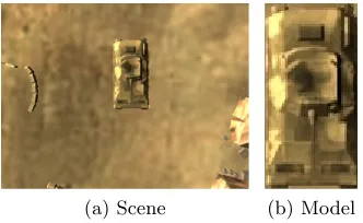
In this test, given a model imageIm , we seek an instance of this model in scene imageIs . This situation can arise when searching for a specific target image in a library of images. It can also arise in an image hand-off scenario where the model is extracted from the image captured by a sensor on one vehicle, and is used as target to be detected in the image captured by a sensor on another vehicle. For example, a model extracted from the image captured by a UAV might then be used as a target to be detected in the scene as captured by a attack device.
Figure 3.8: Detection in Scene Image Is1 using Model Im1 (Image source: Google)
![Figure 3.1: Two (A,B), Three (C) and Four (D) rectangle features. [9]](https://thumb-us.123doks.com/thumbv2/123dok_us/1489511.1182240/37.612.251.375.361.473/figure-b-c-d-rectangle-features.webp)