Managing software performance engineering activities with the performance refinement and evolution model (prem)

Managing Software Performance Engineering Activities with

the Performance Refinement and Evolution Model (PREM)

Chih-Wei Ho

, Laurie Williams

Department of Computer Science, North Carolina State University

1

[email protected],

[email protected]

1. Introduction

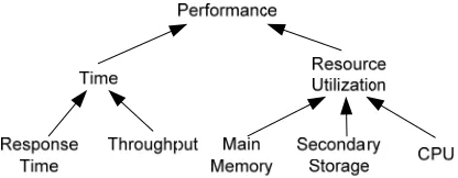
Performance is one of the important non-functional requirements for a software system. A system that runs too slowly is likely to be rejected by all users. Failure to achieve some expected performance level might make the sys-tem unusable, and the project might fail or get cancelled if the syssys-tem performance objective is not met [38]. To build performance into a software system, the development team needs to take performance into consideration through the whole development cycle [13]. Many models, techniques, and methodologies are proposed, trying to address the software performance problems. However, those solutions require different levels of understanding of the performance characteristics. For example, using an unnecessarily complicated performance model during the early stages may require the development team to make assumptions for unknown performance factors. The model may be inaccurate or even useless. The development team needs to choose a proper performance technique, based on the understanding of the performance characteristics, for the technique to provide useful feedback.

In this report, we propose the Performance Refinement and Evolution Model (PREM) to manage software perform-ance development. As shown in Figure 1, PREM is a four-level model, in which a higher level means the better understanding of the performance characteristics. The model shows, at each level, how the performance require-ments and test cases are. With PREM, the development team starts from Level 0 performance requirerequire-ments specifi-cation. Then the team can apply the techniques from PREM-0 to understand the performance characteristics of the system. When more performance characteristics are obtained, the development team can go to a higher PREM level, until the specified requirements are good enough for the project. When applied in different domains, performance requirements can refer to different concepts. Only time-based performance requirements, including response time and throughput, are discussed in this report.

The rest of this report is organized as follows. Section 2 provides the background and related research for PREM; Section 3 describes the metamodel of PREM; Section 4 through 7 present the detail description of PREM; Section 8 concludes the paper and proposes future work; Section 8 gives an illustrative example of how PREM is used to spec-ify a Web application; Section 9 summarizes this

report; Appendix A shows a high-level overview of PREM; Appendix B shows the steps to create per-formance test cases with PREMIER, a perper-formance testing framework that is used in this report; and Ap-pendix C gives the performance requirements for iTrust.

2. Background

This section provides related research and literatures for software performance requirements specification and testing. Information about iTrust, the example application used through this report, is also provided in this section.

2.1. Requirements Specification

PREM-1

PREM-0

PREM-2 PREM-3

Specify qualitative performance requirements Specify quantitative

performance requirements Estimate workloads

Collect workloads

Performance requirements can be specified qualitatively or quantitatively. Quantitative specifications are usually preferred because they are measurable and testable. Basili and Musa advocate that quantitative specification for the attributes of a final software product will lead to better software quality [5]. For performance requirements, Nixon suggests that both qualitative and quantitative specifications are needed, but different aspects are emphasized at dif-ferent stages of development [26]. At early stages, the development focus is on design decisions, and brief, qualita-tive specifications suffice for this purpose. At late stages, quantitaqualita-tive specifications are needed so that the perform-ance of the final system can be evaluated with performperform-ance measurements. PREM follows the same character. At Level 0, requirements are specified qualitatively, while requirements of higher levels are specified later with quanti-tative measurement and workload constraint.

Most software requirements are specified in natural languages [9]. Understanding natural language specifications does not require special training. Therefore, all the stakeholders of the software project can understand the require-ments specified in a natural language. The wide acceptance of specification in a natural language promotes the communication among the stakeholders, and reduces the risk that the stakeholders have different views of the prob-lems that are to be solved with the software under development [22]. However, requirements specified in a natural language can be imprecise [6, 7]. Some approaches have been proposed to detect imprecision in natural language specifications (for example, [12]) or to prevent the introduction of imprecision (for example, [28]).

Formal specifications are precise, and the specified behaviors can be proven mathematically. Among the formal specification languages, the Z notation [17] Vienna Development Method [16] are suitable for functional require-ments, and temporal logics are used in time reasoning for real-time, reactive systems [31]. To read or specify formal requirements, one must be familiar with the specification language. Furthermore, even if the reader knows the specification language, reading or writing formal requirements specification can still be difficult [10]. Several speci-fication patterns are proposed (for example, [11, 21]) as guidance for formal specispeci-fications. Still, formal require-ments specifications are more suitable for automated verification than for human eyes.

In PREM, the choice of language for requirements specifications does not matter. PREM points out the elements that are necessary for precise performance requirements, i.e. subjective efficiency description, performance meas-urements, or workloads. As long as the elements can be found in a specification, a PREM level can be assigned to the specification. On the other hand, if these elements are not found in a specification, the specification is not con-sidered as a performance requirement.

2.2. Performance Testing

Specified workloads, or a collection of requests, need to be generated for performance testing. After the workloads are generated, performance measurements can be collected. The system complies with the performance require-ments if the performance measurerequire-ments meet the expectations stated in the requirerequire-ments specification.

Representative workloads and peak workloads are especially important for software performance testing [39]. Per-formance testing with representative workloads shows how the system performs under regular usage from the users’ perspective. Performance testing with peak workloads provides information about performance degradation under abnormally heavy usage. For a software system, operational profiles can be used as representative workloads [2]. An operational profile of a software system is a complete set of the operations the system performs, with the occur-rence rates of the operations [24]. The occuroccur-rence rates can be obtained from existing business data, or from the information of a previous version or similar systems [25]. If no such information is available, experience shows that the time needed for collecting representative workload data ranges from two to twelve months [1].

At early stages of development, operational profiles or workload data may not be available. In this case, the devel-opment team can use estimation for the workload. Software Performance Engineering (SPE) [35, 37], described in the next subsection, provides a systematic way to estimate the system workloads and performance by building and solving performance models.

2.3. Software Performance Engineering (SPE)

Software Performance Engineering (SPE) [35, 37] is an approach to integrate performance engineering into software development process [3]. In SPE, performance models are developed early in the software lifecycle to estimate the performance and to identify potential performance problems. To make SPE effective, the authors of SPE suggest three modelling strategies [37]:

y Simple-Model Strategy: Early SPE models should be simple and easy to solve. Simple models can provide quick feedback on whether the proposed software is likely to meet the performance goals.

y Best- and Worst-Case Strategy: Early in the development process, many details are not clear. To cope with this uncertainty, SPE uses best- and worst-case estimation for the factors (e.g., resource constraints) that have impact on the performance of the system. If the prediction from the best-case situation is not acceptable, the team needs to find alternative design. If the worst-case performance is satisfactory, the design should achieve the performance goal, and the team can proceed to the next stage of development. If the result is somewhere in between, the model analysis provides information as which part of the software plays a more important role in performance.

y Adapt-to-Precision Strategy: Later in the development process, more software details are obtained. If the in-formation has impact on the performance, it can be added to the SPE models to make the models more precise. SPE uses two types of models: Software execution model, and system execution model. The software execution model characterizes the resource and time requirements. Factors related to multiple workloads, which can affect the software performance, are specified in the system execution model. The software execution model can be easily built, and provide quick feedback on software performance. On the other hand, the system execution model pro-vides analytical results of the system performance under multiple workloads.

In SPE, execution graphs are used to for software execution models. An execution graph specifies the steps in a performance scenario. Execution graphs are presented with nodes and arcs. A node presents a software component, and an arc presents transfer of control. Each node specifies the time required for the step. Graph reduction algo-rithms are used to solve the model and calculate the time needed for the performance scenario. The model presenta-tion and the graph reducpresenta-tion algorithms are defined in [37].

The results from the software execution models are used to derive the parameters for the system execution models. The system execution models are based on queueing network models, showing the hardware and software compo-nents in a system. Performance metrics, including the resource utilization, throughput, and waiting time for the re-quests, can be derived from the system execution models. Automatic tools are available for model analysis [36]. In this paper, we will show how SPE models can be used with PREM.

Table 1 shows how SPE models and techniques fit in PREM. SPE focuses on quantitative performance evaluation, so no PREM-0 techniques are suggested. Performance requirements and testing approaches are not emphasized in SPE, either.

2.4. iTrust

iTrust (http://agile.csc.ncsu.edu/iTrust/) is a web-based medical records application. iTrust was a student term pro-ject for a graduate-level Software Testing and Reliability course at North Carolina State University (NCSU). The

Table 1. PREM levels for SPE models and techniques Level SPE Models and Techniques

PREM-0 N/A

course has a learning objective of combining appropriate testing techniques for the development of a reliable and secure system. The requirements of iTrust are specified by a surgeon in Pennsylvania. A complete list of require-ments can be found at the project web site. In this report, we use iTrust as an example to show how performance requirements and test cases can be developed with PREM.

3. Model Structure

In this section, we provide an overview of PREM1. PREM provides guidelines on the level of detail needed in a performance requirement specification and the corresponding characteristics of test cases. Performance engineering techniques are also classified in PREM levels. Therefore, the development team can analyze the performance using appropriate techniques.

The description of each PREM level is given in this section. The following properties are used to describe each PREM level:

y Starting criteria: A PREM level has one or more starting criteria. The starting criteria show the required prop-erties of the requirements before the techniques at the PREM level can be applied.

y Goal criteria: A PREM level has one or more goal criteria. The goal criteria show the required properties of the requirements for them to be classified as being at a certain PREM level. If a performance requirement satis-fies all the goal criteria of PREM level n, the requirement is called a PREM-n requirement. A performance test case specified based on a PREM-n requirement is called a PREM-n test case.

y Activities: When a requirement satisfies all the entry criteria of a PREM level, and the development team de-cides to achieve the PREM level, the team shall performance the activities for the level. After the activities are successfully performed, the performance requirement specification and related test cases shall satisfy the satis-fying criteria of the PREM level. This paper also provides available techniques for each activity.

y Testing approach: Performance testing shows whether the software system achieves the desired performance goals. The PREM testing approach shows how test cases shall be designed to reflect the performance require-ment of a PREM level. In this report, we use PREMIER2 to demonstrate how performance test cases can be specified. An introduction for PREMIER is provided in Appendix B. The testing approach and PREM are tool-independent. Performance test cases following the test approach can also be specified using other performance testing tools.

4. PREM Level 0

Starting Criteria: Functional requirements are defined in requirements documents.

Goal Criteria: Performance requirements are qualitatively specified in requirements documents.

4.1. Description

PREM-0 represents performance requirements with only qualitative, casual descriptions. An example of PREM-0 requirement is: The Add User process shall be completed quickly. PREM-0 requirements are essentially placehold-ers for future work. By specifying PREM-0 requirements, customplacehold-ers identify the operations for which performance matters. PREM-0 requirements are the starting point which customer and developer will refine or evolve to more precise specifications via PREM-1 or higher requirements.

4.2. Activities

The main activity for PREM-0 is to identify performance requirements. Ideally all the functionalities of a software system should have good performance and consume the least amount of resources. However, in reality, time and budget constraints make this goal infeasible. Additionally, performance goals might conflict with each other. For example, to make a functionality run faster, the development team might use an implementation that consumes more memory. Therefore, the first step toward software performance is to identify which parts of the system require more

1

performance focus. The development team should focus on the requirements for which the performance is sensitive to the users. For example, product search should be responsive for an e-business web site. On the other hand, the efficiency of off-line report generation is not visible from the users’ perspective, and therefore the performance con-cern is less significant.

Informal Approach: Qualitative PREM-0 requirements can be gathered from the discussion with stakeholder such as the user representatives or the marketing department. The development team may ask the users to prioritize the requirements with respect of performance and performance types. The prioritization information shows the parts of the system of which the performance is important to the users.

Performance Requirements Framework (PeRF): PeRF [26] is a framework for performance requirements man-agement for information systems based on the Non-Functional Requirements Framework (NFR Framework) [27]. PeRF provides a systematic way to organize and refine performance requirements, resolve conflicts among require-ments, and justify requirements decisions. PeRF is a qualitative approach that assists the development team to de-cide whether to move toward or away from a requirement. The author of PeRF advocates that in early stages of software development, the focus is on requirements selection from alternatives, and therefore a qualitative approach is more appropriate.

In NFR Framework, a performance goal is represented with the notation: type [topic (parameters)], where type

is a NFR type, and topic (parameters) identifies the requirement. Figure 2, adapted from [26], shows the per-formance requirements types that are used in PREM. For example, Time [Add (User)] means the operation “Add User” has a performance requirements concerning time.

The next step is to refine the performance goals. The goals can be refined by type, topic, or parameter. For example, when refined by type, Time [Add (User)] can be refined to ResponseTime [Add (User)] or Throughput[Add (User)]. When refined by parameter, ResponseTime [Add (User)] can be refined to ResponseTime [Add (Pa-tient)], ResponseTime [Add (HCP)], and so on. When refined by topic, ResponseTime [Add (Patient)] can be refined to ResponseTime [RenderPage (AddPatient)], ResponseTime [ValidateInput (AddPatient)], and

ResponseTime [DatabaseAccess (AddPatient)]. The refinement process and result are presented with a goal graph, which is based on the representation of an and-or tree. Figure 3 shows the refinement for the performance

Figure 2: PREM performance requirements types (adapted from [26])

Time [Add (User)]

ResponseTime

[Add (User)]

Throughput

[Add (User)] X

ResponseTime

[Add (Patient)]

ResponseTime

[Add (HCP)]

ResponseTime

[RenderPage (AddPatient)]

ResponseTime

[ValidateInput (AddPatient)]

ResponseTime

[DatabaseAccess (AddPatient)]

AND AND

goal Time [Add (User)]. Requirements decisions can be made with the goal graph. In this example, the team de-cides to use the response time rather than throughput to specify the performance requirements for Add User, because for iTrust the throughput for this particular functionality is not significant for the users of iTrust. A complete set of refinement rules is presented in [26, 27]. Using PeRF, we can identify that the response time for Add User and Add HCP needs to be short. Further refinements are not visible for the users, and are more appropriate to be documented in performance analysis documents.

4.3. Testing

PREM-0 requirements help the development team focus on the appropriate performance requirements. At this level, brief, high-level performance requirements are sufficient for the team to make high-level, initial requirements deci-sions. A free-form, natural-language-based specification should be used for PREM-0 requirements. Therefore, we do not provide the specification patterns for PREM-0 requirements.

5. PREM Level 1

Starting Criteria: Performance requirements are defined qualitatively in requirements documents. Goal Criteria: y Quantitative requirements are specified in requirements documents.

y Appropriate test cases are specified.

5.1. Description

1 represents performance requirements with quantitatively measurable expectations. An example of PREM-1 requirement is: After the user hits the Add Patient button, the responding Message page shall be rendered within three seconds. Quantitatively measurable specification is the first step to test the requirement in an objective way.

5.2. Activities

The focus of PREM-1 is to specify quantitative requirements and expected performance level for the functionalities of the system. The steps for quantitative performance requirements specification are provided as follows.

5.2.1. Specify Performance Scenarios

A performance scenario describes specific steps involved in a particular software execution that demonstrates cer-tain performance characteristics of the software system. The requirements of iTrust are specified with use cases. A use case has multiple subflows or alternative flows. A scenario is an end-to-end sequence or flow specified in a use case. Performance scenarios are developed from performance requirements identified at PREM-0.

Scenarios can be presented with textual description or graphical models that show the flow of events. For example, the following scenario describes the flow of health care personnel creating a patient in iTrust:

To add a patient in the system, health care personnel click on the “Add Patient” button from the Add Patient page after entering valid information for the patient (as specified in Table x). After the system validates the correctness of the input data, the patient information is stored in the database, and a log entry is generated. Then a message is displayed to inform the user that a new patient has been cre-ated.

5.2.2. Choose performance Metrics

Before a quantitative expectation can be specified, the development team needs to choose a quantitative metric. Table 2 on the next page shows typical performance metrics for different performance types.

5.2.3. Specify Quantitative Requirements

After the performance scenario and metrics are determined, the next step is to specify quantitative expectations. Several sources or approaches can help the team estimate the expectations.

Anecdotal experiences: Anecdotal experiences, although not validated, can give some hint of how well a software system should perform. Table 3 summarizes several Web resources concerning the users’ expectations of the re-sponse time of a Web application. Those numbers can be used as a rough approximation for the performance of a Web application. However, the development team should have more realistic estimations for the system under de-velopment, based on their own team’s experiences and the environments for the software. For example, the most frequent users of iTrust, the medical staff, will most likely access the system from an internal network, and the vali-dation logic for adding a user is not very complicated. Therefore, the response time for adding a user should be very short. After discussion with the users of iTrust, the team and the users agree to set an upper bound of response time of three seconds for adding a user.

Model-based estimation: Performance models may also be used for performance estimations. For example, in Figure 4 in Section 5.2.1, the response time for the scenario can be calculated if we can estimate the time required for each message transition. The performance model breaks the whole scenario into several smaller steps. Estimat-ing the response time for each small step is easier than estimatEstimat-ing the response time for the whole scenario.

There-: User : Add Patient Page : Add Patient Impl : Database

Submit

Validate Data

Insert Patient

Insert Log

Forward to Message Page

[input is correct] Opt

Figure 4: Sequence diagram for the Add Patient scenario

Table 2: Typical performance metrics (adapted from [14])

Performance Type Performance Metrics

Response Time

Transaction processing time Page rendering time Query processing time Resource Consumption

Amount of main memory used Amount of secondary memory used CPU usage

Throughput

fore, especial for a complex scenario, building a performance model can help estimate and set up the performance expectation.

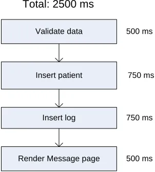
A similar approach is used in the software execution models in SPE [37], although execution graphs are used instead of sequence diagrams. Figure 5 shows the execution graph for the Add Patient scenario. In the call graph, each rec-tangle represents a process step. The estimated time for each step is placed next to the recrec-tangle. In this example, the estimate time for the whole scenario is the sum of the estimate time for each step. In addition to basic rectangle node, other node types, including repetition and case nodes, can also be used in an execution graph. [35, 37] provide detailed description of execution graph and graph reduction rules.

In some situations, the performance requirements are specified before a model is constructed. For example, the cus-tomer may specify that the response time for Add Patient (that is, the duration after the user hits the Add Patient button until the Message page is done rendering) needs to be less than three seconds. The model can help us to de-rive the performance requirements for each step involved in the scenario. For example, the Message page would take 500 milliseconds to render, based on the team’s experience. If the data validation takes less than 500 millisec-onds, then the database operations, including patient and log insertions, can take at most two seconds totally.

To achieve the performance goal of a scenario, each step in the scenario needs to achieve the estimated performance. The performance estimation of each step might be too detailed to be specified in the requirements documents. Such information should be derived during performance analysis, and made available in the design or performance analy-sis documents. Performance test cases can be developed for the small steps. The “performance testing for the small” can help the development team identify the locations of performance problems.

Source Summary

[4]

Provides user expectations for web page loads based on the author’s experience: Fast: under 3 seconds

Typical: 3 – 5 seconds Slow: 5 – 8 seconds Frustrating: 8 – 15 seconds

Unacceptable: more than 15 seconds

[34] Shows the page load times, collected by three leading measurement services: Matrix NetSystems Inc., Keynote Systems, and Gomez, Inc., within the United States.

[33] Shows the time limits for user satisfaction based on the number of elements shown on the screen.

Table 3: Anecdotal experiences of web application performance

Validate data

Insert patient

Insert log

Render Message page Total: 2500 ms

500 ms

750 ms

750 ms

500 ms

5.3. Testing Approach

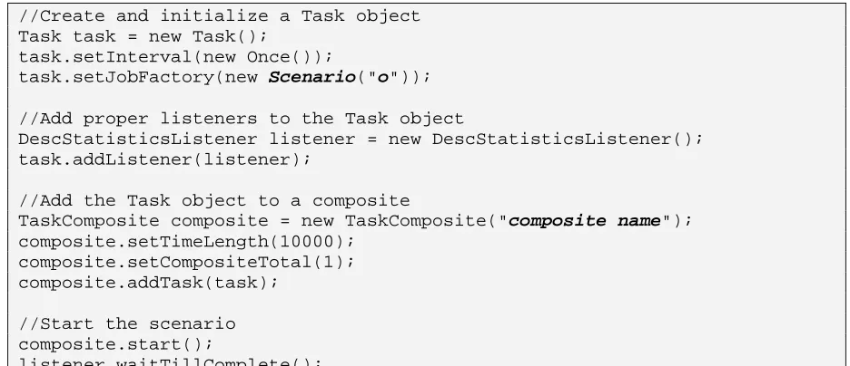
To test that the Add Patient process is completed within two minutes, the tester can use a stop watch to measure the time that is needed for a user to add a patient using the application. Preferably, automated timed tests can also be used to evaluate whether the PREM-1 requirements are met. All the PREM-1 test cases use the code in Figure 6 to set up the workload and initiate the test where the class Scenario, a class that implements the IJobFactory interface, specifies the steps in the performance scenario. The step numbers in the comments indicate the corre-sponding steps to create the test cases as described in Appendix B. The PREM-1 test case runs the scenario once, and takes the time measurement. Although the time length and the total number of requests are specified in the test case, both are ignored if the interval is set to Once. The team may want to run the PREM-1 test cases several time, and calculate the average performance measurements. However, providing that the test case is always run in the same environment, the results from different test runs should be very similar.

//Create and initialize a Task object Task task = new Task();

task.setInterval(new Once());

task.setJobFactory(new Scenario("o"));

//Add proper listeners to the Task object

DescStatisticsListener listener = new DescStatisticsListener(); task.addListener(listener);

//Add the Task object to a composite

TaskComposite composite = new TaskComposite("composite name"); composite.setTimeLength(10000);

composite.setCompositeTotal(1); composite.addTask(task);

//Start the scenario composite.start();

listener.waitTillComplete();

Figure 6: The code that sets up the workload and initiates a PREM-1 test case

6. PREM Level 2

Starting Criteria: Quantitative performance measurements are specified with the requirements.

Goal Criteria: y Estimated average or peak workloads are specified with the requirements in the require-ments docurequire-ments.

y Appropriate test cases are specified.

6.1. Description

PREM-2 represents quantitative performance requirements with estimated workloads for a system. An example of PREM-2 requirement is: The system receives twenty requests every one minute. Among the requests, 5% belong to the Add Patient process. The maximum completion time for 90% of the Add Patient requests shall be below three seconds.

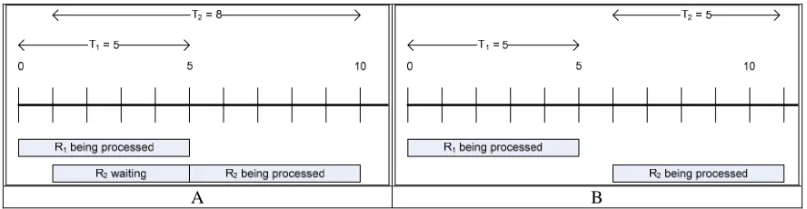
The main activity for PREM-2 is to estimate workloads for the software system. The performance measurement can vary greatly if different workloads are used during performance testing. For example, suppose we have a non-preemptive system that can finish a task in five seconds. In the first scenario, which is shown in Figure 7A, the sys-tem receives a request R1 at time 0, and R2 at the first second. When R2 is sent to the system, the system is

process-ing R1, so R2 needs to be put in a queue until R1 is finished. Therefore, the response time for R2 is eight seconds,

and the average response time for both requests is 6.5 seconds. In another scenario, as shown in Figure 7B, R1 still

comes in at time 0, but R2 arrives at the sixth second. In this case, the response time for R2 is five seconds, making

the average response time 5 seconds.

Several techniques can be used to estimate the system workloads.

Ad-hoc approach: Workloads can be estimated based on the software deployment environment or configuration. For example, in iTrust the users are required to log in the system only once until they log out. Suppose iTrust is deployed in a hospital with 120 medical workers. From the customers, the development team knows that most of the 120 users of iTrust arrive the office between 8:30 to 9:00 and immediately log in. Therefore, we can assume that the request arrival rate for the Log In page is four requests per minute.

Worksheet approach: Joines et al. provide several worksheets in [19] for performance estimation and testing. Some of the worksheets are used to estimate the workloads. Like the ad-hoc approach, the worksheet approach is based heavily on experience and observation. However, the worksheets list the necessary input data (for example, estimate of number of user visits per day and number of hours per day the system is used) and the possible source for the data. Compared to the ad-hoc approach, the worksheet approach is more systematic.

Using existing data: Sometimes the workloads information for a previous release or other similar systems is avail-able. Such information is a good source of workloads estimation for the system under development. Although the system under development may not have exactly the same functionalities as the existing systems, the existing data can give us a good picture of how the system might be used. For example, if a new functionality is designed to re-place two functionalities in the previous release, good workload estimation for the new functionality is the summa-tion of the workloads of the two original ones. If the new funcsumma-tionality is not related to anything in the previous release, other estimation approaches can still be used.

Model-based estimation: Several performance models can be used to evaluate the performance under certain work-loads. For example, queueing network [20] is the basis for system execution model in SPE [37] where a software system is modeled as a network of servers and queues. Some studies demonstrate the possibility of transforming software architecture specifications to queueing-network-based models. For example, Petriu and Shen propose a method to generate layered queueing networks from UML collaboration and sequence diagrams [30]; Cortellessa and Mirandola demonstrate an incremental methodology to transform sequence diagrams and deployment diagrams to extended queueing network models [8]; Menasce and Gomaa present an approach to derive performance models for client/server systems from class diagrams and collaboration diagrams [23]. Petriu and Woodside also show that layered queueing performance models can be generated from software requirements specified with scenario models, including activity diagrams, sequence diagrams, and use case maps [29].

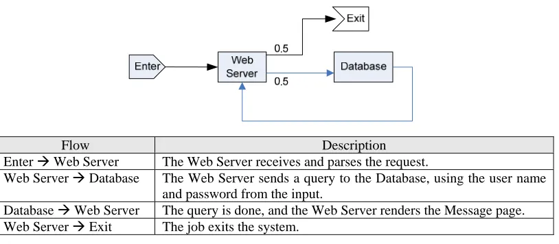
The following example demonstrates how a system execution model can be used to estimate the performance. The Log In scenario is used in this example. To make the example simpler, we assume that the Log In page is already shown on the monitor screen when the user comes in the office and accesses the system. Otherwise, we would need to take the Log In page rendering time and user think time into account, and a more complicated model (in this case, a closed queueing network) would be necessary. Figure 8 shows the queueing network model, where a rectangle represents a server with a queue of infinite length, arrows represent the workflow, and the labels on the arrow are the probabilities of the flows. We can imagine that a job “flows” in the system. When a job flows to the web server, the next step might be querying the database or exiting the system. Therefore, the possibilities for both flows are 0.5 respectively.

To solve the model, we need to identify the throughputs of both servers and the frequency of the incoming requests. As discussed, we estimate the arrival rate for Log In request is four requests per minute, or 0.07 requests per second. From the analysis of PREM-1 models (for example, software execution models), we may identify that the through-puts for the web server (μW) and database server (μD) are 2.00 pages per second and 1.33 queries per second,

respec-tively. Then we can calculate the request rates for the web (λW) and database (λD) servers using the rule that, for

each server, the flow-in rate equals the flow-out rate. That is, for the database server, λD = 0.5 ⋅λW; for the web

server, λW = λD + 0.07. Solving the equations, we can have λD = 0.07 and λW = 0.14.

The next step is to calculate the average number of jobs in the system using the following formula:

∑

=

−

=

i i i

i

L

1

μ

λ

λ

, where k is the number of servers in the queueing network model.

Therefore, the average number of jobs in the system is 0.13. The average response time for Log In is the average number of jobs in the system divided by the request arrival rate, or 0.13 / 0.07 = 1.87 (seconds). That is, if the re-quest rate for Log In is four rere-quests per minute, we may expect an average response time of 1.87 seconds. [32] provides the derivation of the formulas. When the model becomes complicated, calculating the results manually becomes infeasible. Automatic tools such as SPE⋅ED [36] should be used to solve complicated models.

Besides queueing-network-based models, several models may also be used to estimate PREM-2 performance. A nice summary of performance models is provided in [3].

6.3. Testing Approach

To test a PREM-2 requirement, workloads need to be generated according to the workloads estimation. If the distri-bution of the workload is unknown, the workload can be assumed to follow a random process, such as a Poisson process [32]. All the PREM-2 test cases use the code in Figure 9 on the next page to set up the workload and

initi-Flow Description

Enter Æ Web Server The Web Server receives and parses the request.

Web Server Æ Database The Web Server sends a query to the Database, using the user name and password from the input.

Database Æ Web Server The query is done, and the Web Server renders the Message page. Web Server Æ Exit The job exits the system.

ate the test. The classes Scenarion specify the steps in the performance scenarios. The class Dnis an implemen-tation of the IInterval interface, and specifies the distribution for the nth operation described in the requirements. The numbers an, t, and q refer to the parameters of the workload distribution: within t units of time, an% of incom-ing requests belong to operation n. The constant c prevents the test case ends with too few test runs. For example, suppose the estimated workloads specify that one request comes in the system every minute. When using a Poisson process (Dn = ExpInterval) to generate the incoming requests within just one minute, the test case might gener-ate no request at all. However, we may genergener-ate the requests within ten minutes, using the value 10 for the constant c, so that we know some requests are almost certainly generated.

7. PREM Level 3

Starting Criteria: Quantitative performance measurements are specified with the requirements.

Goal Criteria: y Peak or average workloads are collected and specified in the requirements documents.

y Appropriate test cases are specified.

7.1. Description

PREM-3 represents quantitative performance requirements with workloads from collected data. An example of a PREM-3 requirement is “The system is running under the heaviest possible workloads defined in Appendix IV. The average completion time for displaying the promotional message on the mobile tablet after a customer enters a lane where the promotional items are located shall be below 1 second.” At PREM Level-3, the workloads description defines the workloads for different types of requests. If this description is too lengthy or complicated to be specified with the requirement statement, it can be moved to a separate document, such as Appendix IV in this example.

//Step 3: Create and initialize Task objects Task task1 = new Task();

task1.setInterval(new D1());

task1.setPortion(a1 / 100);

task1.setJobFactory(new Scenario1("o1"));

Task task2 = new Task(); Task2.setInterval(new D2());

task2.setPortion(a2 / 100);

task2.setJobFactory(new Scenario2("o2"));

…

//Step 4: Add proper listeners to the Task object

DescStatisticsListener listener = new DescStatisticsListener(); task1.addListener(listener);

//Step 5: Add the Task objects to a composite

TaskComposite composite = new TaskComposite("composite name"); composite.addTask(task1);

composite.addTask(task2);

composite.setTimeLength(t * c); composite.setCompositeTotal(q * c);

//Step 6: Start the scenario composite.start();

listener.waitTillComplete();

7.2. Activities

The focus of PREM-3 is to specify the workloads with collected data. The PREM-3 activities are described as fol-lows.

7.2.1. Collect Representative Workload Data

To test or analyze the average performance for a system, a workload that represents the usage of the system needs to be generated. In a software system, the operational profile [24] can be used to describe the workload of the system [39]. An operational profile of a software system is a complete set of the operations the system performs, with the occurrence rates of the operations [24]. The operational profile can be obtained from several sources:

Existing business data: Market or industrial research reports are available from the government3 or private re-search companies. Those rere-search reports can provide a rough picture of how the software system might be used. The marketing or customer service department in the client organization might have similar data. For example, be-fore iTrust is deployed in the hospital, the health care personnel need to go to the record room if they want to access the medical record. The access log is left on the medical record. After analyzing the record access log, we can un-derstand how often the medical record of a patient is accessed.

Data from previous release or similar applications: If the operational profiles from a previous release or similar applications are available, with a little modification, they can be used for the software under development. From this point of view, it is worthwhile for the team to implement operational profile collecting mechanism in the soft-ware. The next text bullet suggests the data to be collected for operational profiles.

Prototyping or intermediate releases: If no existing data are available, the development team can develop a quick prototype and collect operational profile data from the prototype. For operational profiles, we should collect at least, for each incoming request, the time and the type of the request. Depending on the application, other data might also be relevant. For example, if a user can access an application from the local or external network, the location of the user should be recorded. The development team needs to determine the time and duration of data collection. For example, a shopping web site may need to collect year-round data in order to understand the usage of the web site during the shopping seasons, weekends, and other time. Experiences show that, the time required to collect repre-sentative data ranges from two to twelve months [1]. Therefore, the prototype should be provided as early as possi-ble. In addition to prototypes, we can also use information from intermediate releases, such as alpha or beta ones. However, we need to know who the users are for the intermediate releases, and how different they use the system compared to the target customers [25].

7.3. Testing Approach

The testing approaches for PREM-3 and PREM-2 are similar. The only difference is that, in PREM-3, the workload data are collected from the field. The testing approach for PREM-2 requirements is described in Section 6.3.

8. An Illustrative Example: iTrust

In this section, we demonstrate how PREM is used to design the performance requirements process for iTrust. iTrust is a Web-based medical records application. iTrust was a student term project for a graduate-level Software Testing and Reliability course at North Carolina State University (NCSU). The course has a learning objective of combining appropriate testing techniques for the development of a reliable and secure system. The functional re-quirements of iTrust are specified by a surgeon in Pennsylvania. Use cases are used to describe the functional documents. The length of the functional requirements document is six pages, with eleven use cases. A complete set of functional requirements can be found in the project Web site. The project development time lasted three months, divided into five small iterations. The functionalities of the system are developed incrementally in each iteration. I

3

applied PREM in iTrust to demonstrate that per-formance requirements can be specified and refined with a process following PREM. The resulting performance requirements process for iTrust is shown in Figure 10 in the next page. This section shows how performance requirements are specified with PREM. A complete set of performance re-quirements for iTrust is given in Appendix C.

8.1.

PREM-0 Performance

Re-quirements Specification

Because of the small size of the requirements, we did not use PeRF to identify qualitative requiments. We decided to specify response time re-quirements for user interaction, because response time is the most obvious performance attribute for the users. The only exception is the use case which specifies that an entry is created in the log database whenever a user accesses the system. We refer to this use case as Logging. For the Logging use case, we plan to specify throughput requirements. Several page flow charts were created to show the interactions between the user and the iTrust Web site. Figure 11 shows the page flow chart for the View Records use case, which specifies the steps for patients and health care personnel (HCP) to view a certain type of health records. In the page flow chart, a rectangle represents a Web page, and the links between pages shows the requests that make page transitions. We use two types of re-quests in the page flow chart. The first one is a page request. A page request is a request without immediate input from the user. For example, in Figure 11, the link between Main and Record Type is a page request dubbed “Record Type page.” A page request is usually implemented with a hyper link on a Web page. The other type of request is an

interactive request, which requires some input from the user. For example, in Figure 11 the find “find records ()” links are interactive requests. The input of an interactive request determines the transition of

the page flow. For example, from the Record Query page, if the “find records” is sent with valid input, the page flow will go to the Confirm Record Query page; if invalid input is used with the “find records” request, the page flow will go to the Record Query page. An interactive request is usually implemented with a form on the Web page. In the following sub-sections, we will use the View Records use case to show how the performance requirements are specified and analyzed.

8.2. PREM-1

Performance

Requirements Specification

To analyze the response time for the requests in the page flow chart, we classified the requests into three categories based on the interaction between the Web server and the database server. A simple request is a request that can be handled without the data from the database server. A single-record request is a request that uses, for the purpose of

Figure 12. Sequence diagram for the performance scenario

displaying or input validation, single record from the database. The response time for the request of a single-record request depends on the performance of the database server, but the number of records has little effect. A multi-record request is a request that is involved with multiple records in the database, and the response time depends on the number of records in the database. The types of requests are summarized in Table 4.

After the request types are identified, we estimated the response time for each request. Because iTrust is a Web ap-plication, Internet connection speed plays an important role for the response time experienced by the users. How-ever, the network speed factor depends on the location of the user. We decided to specify the response time for the LAN users (i.e., HCP or other staff who use iTrust in the hospital). According to Sevcilk’s survey [33], users are satisfied with a two-second response time for non-graphic-intensive Web sites. In our experience, for simple re-quests and single-record request, two-second response time can be easily achieved with the hardware specified in the requirements document. Therefore, we specify that the response time limitation for simple and single-record re-quests to be two seconds. However, we were not confident if the multi-record request can satisfy the “two-second rule.” To estimate the response time for the “display record” request, we created a high-level sequence diagram, which is shown in Figure 12.

In the sequence diagram, the user sends the request to the Web server. The Web server then queries the medical records for the patient from the database, renders the Records List page with the query results, and forwards the page

Main

Record Query

Record Type Record List

Record Query page

Record Type page

find records (invalid input)

find records (valid input)

display record

Confirm Record Query find records

(confirmation)

find records (denial)

Figure 11: Page flow chart for the View Records use case

Request Type Requests Total

Simple Request Record Type page; Record Query page; find records

(de-nial); find records (confirmation) 4

Single-Record Request find records (invalid input); find records (valid input) 2

Multi-Record Request display record 1

to the user. The time listed in the diagram is estimated based on our experience under the assumption that the query result returns 50 records. Summing up the time required for each step, the response time for the whole flow is 1.5 seconds, which is safely below two seconds. Therefore, we also specify the response time limitation for the “display record” request to be two seconds.

8.3. PREM-2

Performance

Requirements Specification

Because no existing data are available, we need to estimate how often the system receives a request identified in Table 4. Once again, we use the “display record” request to demonstrate how the workload and response time is estimated. After some observation, we find out that, on average, a HCP finishes the examination in ten minutes (or 600 seconds). During the examination, the HCP needs to view the record once. If the goal is to support one hun-dred HCP on duty, the average request rate for View Records by a HCP is 1/600×100=0.17 requests per second. The response time for View Records can be estimated with an open queueing network model, which is shown in Figure 13. Section 6.2 provides the formula for solving open queueing network models that are used in iTrust per-formance estimation. In the model, each rectangle represents a server with a queue. To solve the model, either manually or with an automatic tool, we need to derive the following parameters from the sequence diagram model.

y Flow probabilities after the Web server: In the HCP Views Records scenario, the Web server is responsible for receiving the requests from HCP, rendering the Records page, and forwarding the Records page to HCP. After the Web server finishes any of these jobs, one of three things might happen: the Web server queries the records from the database; the Web server inserts a log to the database; or the Records page is forwarded to the HCP and the scenario ends. Therefore, after the job leaves the Web server, the probability that the job flows to the database server (p2) is 0.67, and the probability that the job exits the system (p1) is 0.33.

y The throughput of the Web server: Out of the three types of jobs performed by the Web server, two of them take 200 ms (parse the user’s request and forward the Record List page), and the other takes 300 ms (load and render the Record List page). On average, the Web server finishes a job in 2/3×200+1/3×300=700/3 ms = 7 / 30 seconds. Therefore, the throughput for the Web server is 30 / 7 = 4.29 jobs per second.

y The throughput of the database server: The average time for a database server to finish a job is 0.4 seconds. Therefore, the throughput for the database server is 2.5 jobs per second.

y After these parameters are determined, we may solve the model with a tool or with manual computation. The solution shows that the average waiting time for this queueing network is 1.74 seconds, which is still under the two-second response time goal we set up at PREM-1. Therefore, we may update the performance requirement for the “display record” request and add the workload information:

On average, the system receives 0.17 “display record” requests per second from 100 concurrent HCP users. When a HCP submits a “display record” request, the system shall response within two seconds.

For the queueing model to have a solution, the request rate for View Records by a HCP must be lower than 1.23 requests per second. This may be used as peak load estimation. If the peak load or the estimated performance based

on the peak load is not satisfactory to the client, the throughput of the Web or database servers needs to be improved. The improvement can be achieved by, for example, optimizing the implementation or upgrade the hardware.

8.4. PREM-3

Performance

Requirements Specification

We plan to use iTrust as assignments in future Software Testing and Reliability courses. Operational profile data collection mechanism is a requirement for this system, so that the performance requirements can be more specific for future iTrust assignments. When the server receives a request, the user ID, the time and type of the request is logged to the database. The collected data are used to validate the workload estimation. The performance estima-tion using the collected data will be used as the basis of the performance requirements for future iTrust projects.

9. Summary

In this report, I propose a refinement and evolution model for performance requirements, PREM. Using the model as a guideline, a development team can identify and specify PRs incrementally, starting with casual descriptions, and refine them to a desired level of detail and precision. With the specification of performance scenarios, quantitative performance measurements, and average or heaviest workloads, the performance requirements are testable. This model also helps the developers to conduct appropriate performance testing to verify that the software system achieves the desired performance. I also show the performance engineering activities and testing approaches that are suitable for requirements at different PREM levels.

To show the applicability of PREM, I applied PREM on the performance specification for iTrust. In the example, I demonstrate a performance requirements process based on PREM. The performance engineering process is used to specify the performance requirements for iTrust.

References

[1] Avritzer, A., J. Kondek, D. Liu, and E. J. Weyuker, "Software Performance Testing Based on Workload Char-acterization," in Proceedings of the 3rd International Workshop on Software and Performance, pp. 17-24, Rome, Italy, Jul 2002.

[2] Avritzer, A. and E. J. Weyuker, "Generating Test Suites for Software Load Testing," in Proceedings of Inter-national Symposium on Software Testing and Analysis, pp. 44-57, Seatle, WA, Aug 1994.

[3] Balsamo, S., A. D. Marco, and P. Inverardi, "Model-Based Performance Prediction in Software Development: A Survey," IEEE Transactions on Software Engineering, vol. 30, no. 5, pp. 295-310, May 2004.

[4] Barber, S., "Beyond Performance Testing Part 3: How Fast Is Fast Enough?" developerWorks, 2004, Available at http://www-128.ibm.com/developerworks/rational/library/4249.html.

[5] Basili, V. R. and J. D. Musa, "The Future Engineering of Software: A Management Perspective," IEEE Com-puter, vol. 24, no. 9, pp. 90-96, Sep 1991.

[6] Berry, D. M. and E. Kamsties, "Ambiguity in Requirements Specification," in Perspectives on Requirements Engineering, J. C. S. P. Leite and J. Doorn, Eds., Kluwer, 2004, pp. 7-44.

[7] Berry, D. M. and E. Kamsties, "The Syntactically Dangerous All and Plural in Specifications," IEEE Software, vol. 22, no. 1, pp. 55-57, Jan/Feb 2005.

[8] Cortellessa, V. and R. Mirandola, "PRIMA-UML: A Performance Validation Incremental Methodology on Early UML Diagrams," Science of Computer Programming, vol. 44, no. 1, pp. 101-129, Jul 2002.

[9] Denger, C., D. M. Berry, and E. Kamsties, "Higher Quality Requirements Specifications through Natural Lan-guage Patterns," in Proceedings of International Conference on Software: Science, Technology, and Engineer-ing, pp. 80-90, Hertzeliyah, Israel, Nov, 2003.

[10] Dwyer, M. B., G. S. Avrunin, and J. C. Corbett, "Patterns in Property Specifications for Finite-State Verifica-tion," in Proceedings of the 21st International Conference on Software Engineering, pp. 411-420, Los Angeles, CA, May 1999.

[11] Dwyer, M. B., G. S. Avrunin, J. C. Corbett, H. Alavi, L. Dillon, and C. Pasareanu, "A System of Specification Patterns", 2006, Available at http://patterns.projects.cis.ksu.edu/.

[13] Fox, G., "Performance Engineering as a Part of the Development Life Cycle for Large-Scale Software Sys-tems," in Proceedings of The 11th International Conference on Software Engineering, pp. 85-94, Pittsburg, PA, May 1989.

[14] Gao, J. Z., J. H.-S. Tsao, and Y. Wu, Testing and Quality Assurance for Component-Based Software, Norwood, MA, Artech House Publishers, 2003.

[15] Ho, C.-W., M. J. Johnson, E. M. Maximilien, and L. Williams, "On Agile Performance Requirements Specifi-cation and Testing," in Proceedings of Agile 2006 International Conference, pp. 47-52, Minneapolis, MI, Jul 2006.

[16] ISO/IEC, International Standard ISO/IEC 13817-1: Information Technology -- Programming Languages, Their Environments and System Software Interfaces -- Vienna Development Method -- Specification Language -- Part 1: Base Language, 1996.

[17] ISO/IEC, International Standard ISO/IEC 13568: Information Technology Z Formal Specification Notation -- Syntax, Type System, and Semantics, 2002.

[18] ITU, ITU-T Recommendations Z. 120 (04/04) Message Sequence Chart (MSC), 2004.

[19] Joines, S., R. Willenborg, and K. Hygh, Performance Analysis for Java Web Sites, Boston, MA, Addison-Wesley, 2003.

[20] Kleinrock, L., Queueing Systems Volume I: Theory, New York City, New York, Wiley-Interscience, 1975. [21] Konrad, S. and B. H. C. Cheng, "Real-Time Specification Patterns," in Proceedings of 27th International

Con-ference on Software Engineering, pp. 372-381, St. Louis, MO, May, 2005.

[22] Lawrence, B., "Point: Do You Really Need Formal Requirements?," IEEE Software, vol. 13, no. 2, pp. 20, 22, Mar 1996.

[23] Menascé, D. A. and H. Gomaa, "A Method for Design and Performance Modeling of Client/Server Systems,"

IEEE Transactions on Software Engineering, vol. 26, no. 11, pp. 1066-1085, Nov 2000.

[24] Musa, J. D., "Operational Profiles in Software Reliability Engineering," IEEE Software, vol. 10, no. 2, pp. 14-32, Mar 1993.

[25] Musa, J. D., "Chapter 2: Implementing Operational Profiles," in Software Reliability Engineering: More Reli-able Software Faster and Cheaper, 2nd ed. Bloomington, IN, AuthorHouse, 2004, pp. 93-151.

[26] Nixon, B. A., "Managing Performance Requirements for Information Systems," in Proceedings of the 1st In-ternational Workshop on Software and Performance, pp. 131-144, Santa Fe, NM, Oct 1998.

[27] Nylopoulos, J., L. Chung, and B. Nixon, "Representing and Using Nonfunctional Requirements: A Process-Oriented Approach," IEEE Transactions on Software Engineering, vol. 18, no. 6, pp. 483-497, Jun 1992. [28] Ohnishi, A., "Software Requirements Specification Database Based on Requirements Frame Model," in

Pro-ceedings of the 2nd International Conference on Requirements Engineering, pp. 221-228, Colorado Springs, CO, Apr 1996.

[29] Petriu, D. B. and M. Woodside, "Software Performance Models from System Scenarios," Performance Evalua-tion, vol. 61, no. 1, pp. 65-89, Jun 2005.

[30] Petriu, D. C. and H. Shen, "Applying the UML Performance Profile: Graph Grammar-Based Derivation of LQN Models from UML Specifications," in Proceedings of the 12th International Conference on Computer Performance Evaluation: Modelling, Techniques, and Tools, pp. 159-177, London, UK, Apr 2002.

[31] Pnueli, A. and E. Harel, "Applications of Temporal Logic to the Specification of Real Time Systems," Lecture Notes in Computer Science, vol. 311, pp. 84-98, Sep 1988.

[32] Ross, S. M., Introduction to Probability Models, 8th Edition, Burlington, MA, Academic Press, 2003.

[33] Sevcik, P., "How Fast is Fast Enough" Business Communications Review, 2003, Available at http://www.bcr.com/architecture/network_forecasts%10sevcik/how_fast_is_fast_enough?_20030315225.htm. [34] Sevcik, P., "Web Performance -- Not a Simple Number," Business Communications Review, 2003, Available at

http://www.bcr.com/architecture/network_forecasts%10sevcik/web_performance_20030116240.htm. [35] Smith, C. U., Performance Engineering of Software Systems, Reading, MA, Addison-Wesley, 1990.

[36] Smith, C. U. and L. G. Williams, "Performance Engineering Evaluation of Object-Oriented Systems with SPE·ED™," Lecture Notes in Computer Science, vol. 1245, pp. 135-154, 1997.

[37] Smith, C. U. and L. G. Williams, Performance Solutions: A Practical Guide to Creating Responsive, Scalable Software, Boston, MA, Addison-Wesley, 2002.

[38] Sommerville, I., Software Engineering, 7th ed, Boston, MA, Addison-Wesley, 2004.

Appendix A. PREM at a Glance

PREM-0 (Section 4)

Focus: Identify performance requirements. Starting Criteria: Functional requirements are defined.

Goal Criteria: Performance requirements are qualitatively specified in requirements documents. Activities: Identify the performance requirements.

Testing: Qualitative evaluation.

PREM-1 (Section 5)

Focus: Specify quantitative requirements.

Starting Criteria: Performance requirements are defined qualitatively in requirements documents. Goal Criteria: y Quantitative requirements are specified in requirements documents.

y Appropriate test cases are specified. Activities: y Specify performance scenarios.

y Choose performance measurements.

y Specify quantitative requirements.

y Specify PREM-1 performance test cases.

Testing: Run the performance scenario, and take performance measurement.

PREM-2 (Section 6)

Focus: Estimate workloads.

Starting Criteria: Quantitative performance measurements are specified with the requirements.

Goal Criteria: y Estimated average or peak workloads are specified with the requirements in the require-ments docurequire-ments.

y Appropriate test cases are specified.

Activities: y Estimate workloads for different operations.

y Specify PREM-2 test cases.

Testing: Generate multiple asynchronous requests according to the specified workloads. After the requested operations are completed, take performance measurements.

PREM-3 (Section 7)

Focus: Collect workloads data.

Entry Criteria: Quantitative performance measurements are specified with the requirements.

Satisfying Criteria: y PREM-3A: Representative workloads are collected and specified in the requirements documents.

y PREM-3B: Peak workloads are collected and specified in the requirements documents.

y Appropriate test cases are specified.

Activities: y Peak or average workloads are collected and specified in the requirements documents.

y Appropriate test cases are specified.

Appendix B. Writing Performance Test Cases Using PREMIER

PREMIER is a performance testing framework that is designed to work with PREM. Currently PREMIER is avail-able from the SourceForge Subversion repository (https://svn.sourceforge.net/svnroot/premier-spe/trunk/). The class diagram of PREMIER is shown in Figure B1. If the performance requirements are specified using PREM patterns, the requirements can be transformed to corresponding PREMIER test cases. This appendix shows how a PREMIER performance test case is created with JUnit4. The following requirement is used as an example:

The system receives twenty requests every one minute. Among the requests, 5% belong to the Add Pa-tient process. The maximum completion time for 90% of the Add PaPa-tient requests shall be below three second.

Step 1: Use the IJobFactory interface to simulate the scenarios. To implement the IJobFactory interface, the implementing class needs to provide two methods: getJobName() and createNewJob(). The getJobName() method simply returns the identification for the scenario:

public String getJobName() { return "Add Patient"; }

The createNewJob() method creates an instance of Runnable that will be run during performance testing. We use HTTPUnit5 to simulate a web browser at the user’s end. To specify the scenario with HTTPUnit, the devel-opment team may list the steps that are required in the scenario:

1. Go to the index page (URL: http://internal.virtualmed.com/itrust/index.jsp).

2. In the log in form, fill in the MID (9000000003) and password (1xb567H). Click on the Login button. 3. Select the Add Patient action (URL: http://internal.virtualmed.com/itrust/addPatient.jsp).

4. Fill in the patient information (as specified in table n in Appendix IV). 5. Click on the Add Patient button.

We are interested in the performance of the last step. Therefore, only the last step needs to be included in the re-turned Runnable object. The code to simulate the scenario is as follows.

public Runnable createNewJob() {

final WebConversation wc = new WebConversation(); final WebRequest indexPage = new GetMethodWebRequest(

"http://internal.virtualmed.com/itrust/index.jsp"); final WebRequest addPatientPage = new GetMethodWebRequest(

"http:// internal.virtualmed.com/itrust/addPatient.jsp");

4

http://www.junit.org

5

http://httpunit.sourceforge.net/

TaskComposit

+ TimeLength + CompositeTotal

+ start ( )

Task *

«interface»

ITaskListener

*

«interface»

IInterval

1

«interface»

IJobFactory

1

«interface»

Runnable

final WebForm addPatientForm;

try{

WebResponse logInRes = wc.getResponse(indexPage); WebForm logInForm = logInRes.getForms()[0];

logInForm.setParameter("mid", "9000000003"); logInForm.setParameter("pw", "1xb567H"); logInForm.submit();

WebResponse addPatientPageRes = wc.getResponse(addPatientPage); addPatientForm = addPatientPageRes.getForms()[0];

addPatientForm.setParameter("userType", "1");

addPatientForm.setParameter("formIsFilled", "true"); …

} catch (Exception e) {

throw new RuntimeException(e); }

return new Runnable() { public void run() {

try {

addPatientForm.submit(); } catch (Exception e) {

throw new RuntimeException(e);

} }

}; }

Step 2: Create a JUnit test class. The following code shows an empty JUnit test method in a test class. In the rest of the steps, we will work on the test method.

public class AddPatientPerformanceTest extends TestCase { public void testAddPatientResponseTime() {

} }

Step 3: Create and initialize a Task object. In PREMIER, Task is the class that creates and runs the Runnable objects specified in IJobFactory. We need to specify the request ratio, the request distribution, and the job fac-tory for the Task object. In this example, because the requirement does not specify the distribution of the incoming request, we use a Poisson process.

Task addPatientTask = new Task();

addPatientTask.setInterval(new ExpInterval()); addPatientTask.setPortion(0.05);

addPatientTask.setJobFactory(new AddPatientScenario());

Step 4: Add proper listeners to the Task object. The listeners can monitor the progress of the scenario. In this example, we want to know whether more than 90% of the Add Patient requests can be completed within three sec-onds. The DescStatisticsListener, which calculates descriptive statistics for the tasks, can provide such information. DescStatisticsListener listener = new DescStatisticsListener();

addPatientTask.addListener(listener);

Task. We need to specify the length of the test time and the total number of requests in the composite object. In this example, Add Patient only accounts for 5% of the incoming requests. If we want to run the Add Patient sce-nario 10 times statistically6, we will need 200 incoming requests. Because the requests arrival rate is 20 requests per minute, we need to run a ten-minute long test. If we have other scenarios (Task objects), we may add them to the same composite object. PREMIER will generate a workload that consists of all the Task objects in the composite. TaskComposite composite = new TaskComposite("Add Patient");

composite.setTimeLength(600000); //10 minutes composite.setCompositeTotal(200);

composite.addTask(addPatientTask);

Step 6: Start the scenario and take performance measurements. Invoking the start() method of the composite will start all the tasks that are added to the composite object. The listener has a method, waitTillComplete(), that will cause the test to wait until all the requests are completed. After the requests are completed, the listener has the performance measurements. In this example, we want to make sure that more than 90% of the requests are com-pleted within three seconds.

composite.start();

listener.waitTillComplete();

assertTrue(listener.getSuccessRate(3000) > 0.9);

6

Appendix C. Performance Requirements for iTrust

This appendix provides the performance requirements for iTrust, following the PREM process as shown in Figure 10. A response time requirement is given for each of the page transition. Each page transition is a result of a re-quest of the user. As described in Section 8.2, the page transitions are classified into three categories: simple rere-quest, single-record request, and multi-record request. For single-record requests and multi-record requests, an additional database access, an additional database access is necessary if log entries are to be put in the database. For the multi-record requests, we assume that the number of multi-records is 50. For some requests, the number of multi-records can be much larger than 50. We describe the performance of these requests in special cases. The first part of this appendix shows the page flow diagrams and the request types for each use case except for Use Case 4. Use Case 4 describes the format for the transaction log, and has no page flow associated with the use case. Sections C.2 and C.3 show how PREM-1 and PREM-2 performance requirements are specified. For the discussion of PREM-0 (qualitative descrip-tion) and PREM-3 (workload collecdescrip-tion) performance requirements, please read Sections 8.1 and 8.4 respectively.

C.1. Page Flow Diagrams and Request Types

C.1.1. Use Case 1: Create and Disable Patients and Health Care Personnel

Main

Create User

Review Create User

Message Disable

User

Review Disable User

Activate Authorized Personnel

Confirm Activation Create User

page

create user (invalid input)

create user (valid input)

create user (denial)

create user (confirmation)

Disable User page

disable user (invalid input)

disable user (valid input)

disable user (denial)

disable user (confirmation)

Activate AP page

activate AP (invalid input)

activate AP (valid input)

activate AP (denial) activate AP (confirmation)

Request Type Requests

Simple Request

Create User page, Disable User page, Activate AP page, create user (denial), disable user (denial), activate AP (de-nial)

Single-Record Request without no other DB access

create user (invalid input), create user (valid input), dis-able user (invalid input), disdis-able user (valid input), acti-vate AP (valid input), actiacti-vate AP (invalid input)

Single-Record Request with one additional DB access