An Alternation Diffusion LMS Estimation Strategy over Wireless
Sensor Network
Lin Li* and Donghui Li
Abstract—This paper presents a distributed estimation strategy called alternation diffusion LMS estimation (AD-LMS) to estimate an unknown parameter of interests from noisy measurement over wireless sensor network. It is useful in the wireless sensor networks where robustness and low consumption are desired features. Diffusion LMS is introduced in this estimation strategy to improve the performance and reduce the communication burden. With the proposed strategy, whether each node distributes its estimation depends on an alternative parameter. The node only exchanges its estimation when the instant time meets some conditions. Next, each node combines the estimations of neighbors with its own estimation using combination coefficients upon the topology of the network. At last, the nodes update their estimations with a normalized LMS algorithm. The proposed AD-LMS strategy is compared to standard diffusion strategy. The results show that they achieve exactly the same coverage rate and nearly the network performance (network MSD and steady-state MSD) of standard diffusion strategy while reducing the communication burden significantly.
1. INTRODUCTION
In a wireless sensor network, the nodes collect data in a distributed way in some applications such as target localization and tracking, environment monitoring, spectrum sensing, and automotive radars [1]. An unknown common parameter of interest is the distortion of the collected regression data by noise, which occurs when the local copy of the underlying system input signal at each node is corrupted by various sources of impairment such as measurement or quantization noise [2]. A big problem is how to estimate the unknown parameter from the obtained data from each node in a WSN [3].
To solve the problem of the parameter estimation in a WSN, there have been two main strategies in recent years: one is centralized strategy, and the other is distributed strategy [4]. In a centralized strategy, all the nodes need to send their estimations to a central node to process and estimate the unknown parameter. The central node can offer an estimation after obtaining the whole information of the network. However, a network with this strategy increases the cost greatly. The power of sensor node which is usually supplied by battery runs out quickly by using the centralized strategy, and this is unacceptable. Since the WSNs are limited with energy, and the connection between nodes are multi-hop, distributed strategies have attracted more and more attention. In a distributed strategy, each node estimates the parameter based on its own local computation and the estimation information received from its neighbors without the help of the central node [5]. The existing distributed strategies can be classified into incremental [6, 7], diffusion [2, 8–11] and hierarchical strategies [12, 13]. The diffusion LMS strategy is the most popular strategy, and we focus on it in this paper. Each node performs an LMS update after exchanging the estimation with its neighbors in a diffusion strategy [9]. Compared with the centralized strategy, it can achieve scalability, robustness and low communication burden. There are many distributed diffusion strategies proposed in the past papers. In work [8], a simple
Received 23 April 2018, Accepted 29 June 2018, Scheduled 13 July 2018
* Corresponding author: Lin Li ([email protected]).
adaptive diffusion LMS strategy is illustrated. [9] analyses the performance of CTA, and ATC diffusion strategy in a distributed network [11] uses the normalize step-size in the adaptive stage to adapt the input signal. Shao et al. [14] propose a robust diffusion estimation algorithm based on a minimum error entropy criterion with a self-adjusting step-size to gain a fast speed of convergence. As most networks contain a large number of nodes and a complex topology, the communication burden of estimation is still considerable in a distributed diffusion strategy. The broken-motifs diffusion LMS (BM-LMS) algorithm [15] reduces the communication burden with only a subset of edges which are participated in communications.
Considering the communication burden in a distributed network, we propose a new distributed estimation strategy, called alternation diffusion LMS estimation (AD-LMS). In this paper, each node distributes its estimation depending on an alternative parameter. The node only exchanges its estimation when it is chosen. Next, each node combines the estimations from other nodes with its own estimation using combination coefficients upon the topology of the network. At last, each node performs an LMS update of estimation with a normalized step-size. Moreover, by using the proposed AD-LMS strategy, the communication burden in the whole network has been significantly reduced with a little influence on the network performance.
The paper is organized as follows. In Section 2, we state the estimation problem and define the cost functions. Then, the derivation of the diffusion solution strategy is presented. In Section 3, we describe our AD-LMS strategy. In Section 4, we provide detailed simulation results of a distributed network with 50 nodes to illustrate the performance of our strategy compared with the existing diffusion strategies. In Section 5 we have a conclusion of this paper.
2. PROBLEM STATEMENT
2.1. Network Model
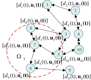
In this paper, we consider a WSN with N nodes. A typical topology of the WSN is illustrated in Fig. 1. The nodes are denoted by neighbors as they can exchange their information directly without transferring. A usual linear regression model [16] is shown as follows:
di(t) =wToui(t) +vi(t) (1)
The node i outputs a scalar measurement di(t) at instant time t which relates to the input regression vector ui(t) and the true parameter wo, where di(t) is a scalar value. ui(t) is an M ×1 vector so is
wo. vi(t) denotes the observation noise or disturbance of each node I, and vi(t) is independent and
unrelated. We assume thatvi(t) of each node I at instant timetis a random signal with zero mean and
varianceσ2
v,i.
1
8
3
6 7
4
5
9 10 2
7
Ω
7 7
[d (t),u (t)]
1 1
[ (t),d u (t)] [d2(t),u (t)2 ]
3 3
[d (t),u (t)]
4 4
[d (t),u (t)]
5 5
[d (t),u (t)]
6 6
[d (t),u (t)]
8 8
[d (t),u (t)]
9 9
[d (t),u (t)]
10 10
[d (t),u (t)]
2.2. Cost Function
To achieve an estimation vector wforwo, the global cost function [16] of the whole network should be
minimized given by
Jglobal(w) =
N
i=1
Edi(t)−uTi (t)w2 (2)
where E denotes the expectation operator. Assume that the processui(t) is jointly wide sense stationary. A centralized least mean square (LMS) algorithm update [17] is shown as
w(t + 1) =w(t) +μ
N
i=1
ui(t)(di(t)−uTi (t)w(t)) (3)
whereμ >0,μ is a step size, andw(t) is the estimation ofwo in time t.
2.3. Distributed Diffusion Strategy
By the centralized LMS algorithm, the whole network information should be collected and processed in a central node. To send and transmit the information to central node, the communication burden is greatly increased [18]. It is impractical in a WSN due to the limited resources of nodes. Moreover, if there are some link failures and changes in the network, the centralized algorithm will not have a good performance [19].
On the contrary, we introduce the distributed diffusion strategy to overcome these drawbacks. In a distributed estimation strategy, each node only needs to exchange the information with its neighbors to achieve the estimation. It is assumed that two nodes are connected if they can communicate with each other directly [10]. The neighbor denoted by Ωi of node i is a set of nodes (include node i itself) which are connected with node i. Each node can process its local estimation and get the diffusion estimations from its neighbors. In Fig. 1, there is an example of a network consisting of ten nodes. The arrows indicate the connections of the nodes while the nodes at the end of an arrow can exchange information with each other. The neighbor of node 7 denoted by Ω7 includes nodes 5, 6, 7, 8. In this case, the
distributed estimation does not collapse even if some nodes fail.
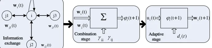
The distributed strategy is commonly performed in two stages: adaption and combination. Based on the topology of the network, the estimations are combined with combination coefficients.
γii+
j∈Ωi
γij= 1 j= i (4)
where γii is the combination coefficient of itself, and the γij is the combination coefficient of node j in
its neighbors, satisfying Eq. (4). In this paper we use the Metropolis rules [20] to get the combination coefficients with Eq. (5).
⎧ ⎪ ⎪ ⎪ ⎪ ⎨ ⎪ ⎪ ⎪ ⎪ ⎩
γij=
1
max(|Ωi|,|Ωj|) if j∈Ωi j= i
γij= 0 if j∈/ Ωi j= i
γii= 1−
j∈Ωi
γij if j∈Ωi j= i
(5)
where|Ωi|denotes the cardinality of the set Ωi.
In this paper, we seek to estimate the parameter of wo only by processing the information of the
neighbors in a distributed diffusion strategy. Node i has a priori estimatewi(t) of parameter wo in the
instant time t. The update function is generated in Eq. (6).
wi(t + 1) = arg min
wi
γiiwi−wi(t)2+ j∈Ωi,i=jγijwi−wj(t)2+μi(di(t)−uTi (t)wi)2
(6)
To simplify the update function, we expand the last item (di(t)−uTi (t)wi)2 of the unknown wi
aroundwj(t) in Taylor formula.
(di(t)−uTi (t)wi)
2=
e2ij(t)−2eij(t)uTi (t)(wi−wj(t)) +owi2 (7)
whereeij(t) =di(t)−uTi (t)wj(t).
In the same way, the expansion of the last term aroundwi(t) is Eq. (8).
(di(t)−uTi (t)wi)2=e2i(t)−2ei(t)uTi (t)(wi−wj(t)) +owi2 (8)
whereei(t) =di(t)−uTi (t)wi(t).
Then, we put Eqs. (7) and (8) into Eq. (6). Since the combination coefficients satisfy Eq. (4), we have the function in Eq. (9).
wi(t + 1) = arg min
wi ⎧ ⎪ ⎪ ⎪ ⎪ ⎪ ⎨ ⎪ ⎪ ⎪ ⎪ ⎪ ⎩
γiiwi−wi(t)2+
j∈Ωi,i=j
γijwi−wj(t)2
+μiγii[e2i(t)−2ei(t)uTi (t)(wi−wi(t))]
[e2ij(t)−+μiγij
j∈Ωi,i=j
2eij(t)wj(t)uTi (t)(wi−wj(t))]
⎫ ⎪ ⎪ ⎪ ⎪ ⎪ ⎬ ⎪ ⎪ ⎪ ⎪ ⎪ ⎭
(9)
The term within the large braces is a function of wi. To get wi(t + 1), we differentiate the function of
wiand let it equal to 0. Then the distributed update estimation wi(t + 1) is shown in Eq. (10).
wi(t + 1) =ϕi(t + 1) +μiui(t)(di(t)−uTi (t)ϕi(t + 1)) (10)
where
ϕi(t + 1) =γiiwi(t) +
j∈Ωi,i=jγijwj(t) (11)
Eq. (11) is regarded as the combination stage, and Eq. (10) is the adaptive stage. The distributed diffusion LMS is shown in Fig. 2.
i(t)
w
j3 j1
j2 i
j1(t)
w
j2(t) w
j3(t) w
Information Information exchange exchange
i(t)
w
j(t)
w
ij γ
Σ
ii γ
i(t 1)
ϕ +
Combination Combination
st stage
i u (t)
( ) i
d t
i(t 1)+ w
Adaptive Adaptive
stage stage
i(t 1)
ϕ +
Figure 2. Distributed diffusion strategy.
3. THE PROPOSED AD-LMS STRATEGY
By the strategy in Section 2, the amount of information exchange is reduced. However, the communication burden is still considerable in WSN. If a node updates its estimation all by itself without cooperation, the network performance is bad which cannot meet the requirement of estimation. Then, we propose our AD-LMS to balance the network performance and communication burden.
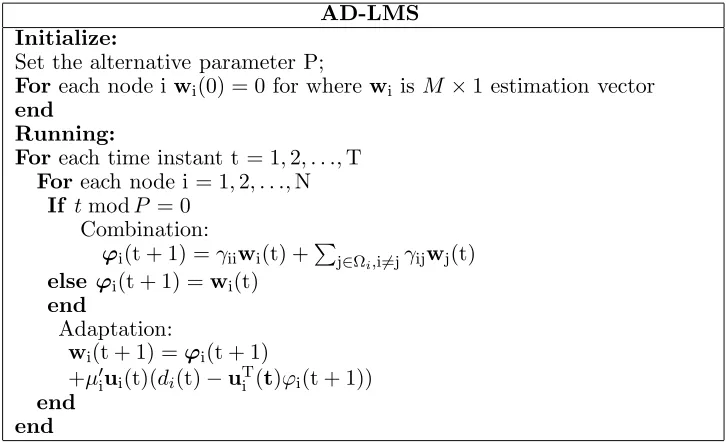
In other words, the node only needs to exchange its estimation when the instant time “t mod P = 0” which means that it is chosen. With the AD-LMS strategy, the communication burden is 1/P of that in the standard diffusion strategy. Since the performance of the LMS algorithm strongly depends on the step size parameterμ, the normalized algorithm is used in this paper. We useμi=μi/uTi (t)ui(t)
instead of μi. The AD-LMS strategy is illustrated in detail in Table 1.
Table 1. AD-LMS strategy.
AD-LMS Initialize:
Set the alternative parameter P;
For each node iwi(0) = 0 for where wiis M×1 estimation vector
end Running:
For each time instant t = 1,2, . . ., T
For each node i = 1,2, . . ., N
If tmodP = 0 Combination:
ϕi(t + 1) =γiiwi(t) + j∈Ωi,i=jγijwj(t)
else ϕi(t + 1) =wi(t)
end
Adaptation:
wi(t + 1) =ϕi(t + 1)
+μiui(t)(di(t)−uTi (t)ϕi(t + 1))
end end
0 10 20 30 40 50 60 70
0 10 20 30 40 50 60 70
80 Network Toplogy
1 1 1 1 1 1 1 1 1 1 1 1 1 1 1 1 1 1 1 1 1 1 1 1 1 1 1 1 1 1 1 1 1 1 1 1 1 1 1 1 1 1 1 1 1 1 1 1 1
1 2222222222222222222222222222222222222222222222222 333333333333333333333333333333333333333333333333
4 4 4 4 4 4 4 4 4 4 4 4 4 4 4 4 4 4 4 4 4 4 4 4 4 4 4 4 4 4 4 4 4 4 4 4 4 4 4 4 4 4 4 4 4 4 4 5 5 5 5 5 5 5 5 5 5 5 5 5 5 5 5 5 5 5 5 5 5 5 5 5 5 5 5 5 5 5 5 5 5 5 5 5 5 5 5 5 5 5 5 5 5 6 6 6 6 6 6 6 6 6 6 6 6 6 6 6 6 6 6 6 6 6 6 6 6 6 6 6 6 6 6 6 6 6 6 6 6 6 6 6 6 6 6 6 6 6 77777777777777777777777777777777777777777777 8 8 8 8 8 8 8 8 8 8 8 8 8 8 8 8 8 8 8 8 8 8 8 8 8 8 8 8 8 8 8 8 8 8 8 8 8 8 8 8 8 8 8 9 9 9 9 9 9 9 9 9 9 9 9 9 9 9 9 9 9 9 9 9 9 9 9 9 9 9 9 9 9 9 9 9 9 9 9 9 9 9 9 9 9 10 10 10 10 10 10 10 10 10 10 10 10 10 10 10 10 10 10 10 10 10 10 10 10 10 10 10 10 10 10 10 10 10 10 10 10 10 10 10 10 10 11 11 11 11 11 11 11 11 11 11 11 11 11 11 11 11 11 11 11 11 11 11 11 11 11 11 11 11 11 11 11 11 11 11 11 11 11 11 11 11 12 12 12 12 12 12 12 12 12 12 12 12 12 12 12 12 12 12 12 12 12 12 12 12 12 12 12 12 12 12 12 12 12 12 12 12 12 12 12 13 13 13 13 13 13 13 13 13 13 13 13 13 13 13 13 13 13 13 13 13 13 13 13 13 13 13 13 13 13 13 13 13 13 13 13 13 13 14141414141414141414141414141414141414141414141414141414141414141414141414 15 15 15 15 15 15 15 15 15 15 15 15 15 15 15 15 15 15 15 15 15 15 15 15 15 15 15 15 15 15 15 15 15 15 15 15 16 16 16 16 16 16 16 16 16 16 16 16 16 16 16 16 16 16 16 16 16 16 16 16 16 16 16 16 16 16 16 16 16 16 16 17171717171717171717171717171717171717171717171717171717171717171717
18 18 18 18 18 18 18 18 18 18 18 18 18 18 18 18 18 18 18 18 18 18 18 18 18 18 18 18 18 18 18 18 18 19 19 19 19 19 19 19 19 19 19 19 19 19 19 19 19 19 19 19 19 19 19 19 19 19 19 19 19 19 19 19
19 20202020202020202020202020202020202020202020202020202020202020 212121212121212121212121212121212121212121212121212121212121 22 22 22 22 22 22 22 22 22 22 22 22 22 22 22 22 22 22 22 22 22 22 22 22 22 22 22 22 22 23 23 23 23 23 23 23 23 23 23 23 23 23 23 23 23 23 23 23 23 23 23 23 23 23 23 23 23 24 24 24 24 24 24 24 24 24 24 24 24 24 24 24 24 24 24 24 24 24 24 24 24 24 24 24 2525252525252525252525252525252525252525252525252525
26 26 26 26 26 26 26 26 26 26 26 26 26 26 26 26 26 26 26 26 26 26 26 26 26 27 27 27 27 27 27 27 27 27 27 27 27 27 27 27 27 27 27 27 27 27 27 27 27 28 28 28 28 28 28 28 28 28 28 28 28 28 28 28 28 28 28 28 28 28 28 28 29 29 29 29 29 29 29 29 29 29 29 29 29 29 29 29 29 29 29 29 29 29 30 30 30 30 30 30 30 30 30 30 30 30 30 30 30 30 30 30 30 30
30 3131313131313131313131313131313131313131 32323232323232323232323232323232323232 3333333333333333333333333333333333333434343434343434343434343434343434 35353535353535353535353535353535 36 36 36 36 36 36 36 36 36 36 36 36 36 36 36 37 37 37 37 37 37 37 37 37 37 37 37 37
37 38383838383838383838383838
39 39 39 39 39 39 39 39 39 39 39 39 40 40 40 40 40 40 40 40 40 40
40 41414141414141414141
42 42 42 42 42 42 42 42 42 43 43 43 43 43 43 43
43 44444444444444
45 45 45 45 45 45 46 46 46 46 46 47 47 47 47 48 48 48 49 49 50
Figure 3. WSN topology.
4. SIMULATION RESULTS
0 5 10 15 20 25 30 35 40 45 50
Nodes number i
11.5 12 12.5 13 13.5 14 14.5 15
Tr(R
i
)
Figure 4. Trace of regressors.
0 5 10 15 20 25 30 35 40 45 50
Nodes number i 9
9.2 9.4 9.6 9.8 10 10.2 10.4 10.6 10.8
Noise variance
v,
i
2
10-4
Figure 5. Noise variance.
N = 50 nodes. Communication burden covers number of transmitted packets, packet delivery ratio, data delay, or processing load. Since the packet delivery ration and data delay are the same as other LMS strategies. There should be a positive correlation between the number of transmitted packets and the processing load. We use the number of transmitted packets to evaluate the communication burden compared with other strategies as in [9, 15]. The red asterisks represent the sensor node, and the blue lines represent the communication link within the network. In our simulation, we use the input regressors of each node which are generated as sample vectorsui,t= [ui(t)ui(t−1). . . ui(t−M+1)]T of an AR-1 [21] process of the formui(t) =xi(t)+ρiui(t−1) whereρi= 0.5 is a correlation coefficient,
and xi(t) is a white noise process with σx,i= 1. The parameter M is set to 10, and the input regression
vector ui,t is with 10 dimensions. The trace of each node’s regression matrix Ri = E(ui(t)uTi (t)) is
shown in Fig. 4. The noise inputvi(t) at each node is zero-mean Gaussian, and we show the variant of
each node’s noise in Fig. 5. The input regressors and noise are temporary and spatially independent of each other.
The step size of LMS without cooperation, standard diffusion LMS and our ADLMS is set μ= 0.4/uTi (t)ui(t). We can set the alternative parameter from 1 to I + 1. AD-LMS strategy is the
same as the LMS without communication when P = I + 1, and it is the same as standard DLMS when P = 1. In our simulation, the alternative parameter of AD-LMS strategy is set to 2, 5, 8 to compare with other strategies. All the curves shown in the figures are the average results of 50 independent runs. To evaluate each strategy, we use mean-square deviation (MSD) of the whole network defined as MSD(dB)= 20log(N1EW(t)−Wo2), shown in Fig. 6. At instant time 300, the network MSD of the
proposed AD-LMS and standard diffusion is below−40 dB while the LMS without cooperation strategy is about−35 dB. The standard DLMS has the best MSD performance, and the MSD of AD-LMS with P = 2 is near the standard one. With P increasing, the network MSD performance is worse. The convergence rates of all the strategies are exactly the same.
To evaluate the performance in the steady state, we average the data of the last 500 instant times as a steady state. In this paper, we define the steady-state MSD of node i as MSDi(dB) = 20log(Ew−wi(t)2). In Fig. 7, the steady-state MSD of AD-LMS with P = 2,5,8
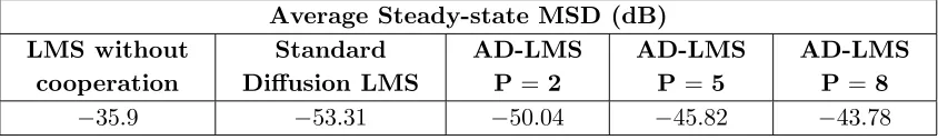
is about −50 dB, −46 dB, −44 dB. The MSD of standard DLMS is about-53 dB, and the no-diffusion strategy is about −36 dB. Table 2 illustrates the comparison of average steady-state MSD per node. When P = 2,5,8, respectively, the AD-LMS gain 94.3%, 84.4%, and 82% MSD performance of standard DLMS.
0 200 400 600 800 1000 1200 1400 1600 1800 2000
time
-70 -60 -50 -40 -30 -20 -10 0 10
MSD (dB)
LMS without cooperation standard DLMS AD-LMS P=2 AD-LMS P=5 AD-LMS P=8
Figure 6. Network MSD.
5 10 15 20 25 30 35 40 45 50
Nodes number i
-52 -50 -48 -46 -44 -42 -40 -38 -36
Steady state MSD
i
(dB)
LMS without cooperation standard DLMS AD-LMS P=2 AD-LMS P=5 AD-LMS P=8
Figure 7. Steady-state MSD.
Figure 8. Average number of transmitted packets per time.
parameter. Fig. 8 shows the average number of transmitted packets per time. The average number in standard DLMS is 25000. As the node does not exchange the estimation all the time, the number of AD-LMS with P = 2,5,8 is respectively 12500, 5000 and 3125.
Since the standard diffusion strategy has a heavy communication burden in the WSN, and the network performance by using the LMS strategy without cooperation cannot meet the requirement of estimation, our AD-LMS strategy reduces the communication burden significantly. Table 3 shows the comparison of communication burden with standard diffusion strategy and AD-LMS with the alternative parameters in this simulation. By the AD-LMS, the network performance and communication are balanced. We can set the alternative parameter depending on which one is more concerned in a specific network.
Table 2. Average steady-state MSD comparison.
Average Steady-state MSD (dB) LMS without
cooperation
Standard Diffusion LMS
AD-LMS P=2
AD-LMS P= 5
AD-LMS P =8
Table 3. Communication burden comparison.
Communication burden
Standard Diffusion LMS AD-LMS P =2 AD-LMS P=5 AD-LMS P=8
100% 50% 20% 12.5%
5. CONCLUSION
In this paper, a distributed estimation strategy denoted by alternation diffusion LMS estimation (AD-LMS) for WSN is proposed to estimate an unknown parameter with less communication burden. We describe the diffusion LMS in a WSN and the derivation of the algorithm. Since the communication burden is still high in the standard diffusion way, we propose our AD-LMS. With an alternative parameter, each node only needs to exchange its estimation in some specific instant times. Hence the communication burden decreases considerably. Compared with the standard diffusion strategy, the same coverage rate is achieved with a little influence on MSD performance. Through setting the alternative parameter of the AD-LMS, we can balance the network performance and network communication burden.
REFERENCES
1. Rahman, M. U., “Performance analysis of MUSIC DOA algorithm estimation in multipath environment for automotive radars,” International Journal of Applied Science & Engineering, Vol. 14, 125–132, 2016.
2. Abdolee, R. and B. Champagne, “Diffusion LMS strategies in sensor networks with noisy input data,” IEEE/ACM Transactions on Networking, Vol. 24, 3–14, 2015.
3. Lopes, C. G. and A. H. Sayed, “Incremental adaptive strategies over distributed networks,” IEEE
Transactions on Signal Processing, Vol. 55, 4064–4077, 2007.
4. Liu, Y., C. Li, W. K. S. Tang, and Z. Zhang, “Distributed estimation over complex networks,”
Information Sciences, Vol. 197, 91–104, 2012.
5. Arablouei, R., Y. F. Huang, S. Werner, and K. Do˘gan¸cay, “Reduced-communication diffusion LMS strategy for adaptive distributed estimation,”Signal Processing, Vol. 117, 355–361, 2014.
6. Sahoo, U. K., G. Panda, B. Mulgrew, and B. Majhi, “Robust incremental adaptive strategies for distributed networks to handle outliers in both input and desired data,”Signal Processing, Vol. 96, 300–309, 2014.
7. Cattivelli, F. S. and A. H. Sayed, “Analysis of spatial and incremental LMS processing for distributed estimation,” IEEE Transactions on Signal Processing, Vol. 59, 1465–1480, 2011. 8. Lopes, C. G. and A. H. Sayed, “Diffusion least-mean squares over adaptive networks: Formulation
and performance analysis,” IEEE Transactions on Signal Processing, Vol. 56, 3122–3136, 2008. 9. Cattivelli, F. S. and A. H. Sayed, “Diffusion LMS strategies for distributed estimation,” IEEE
Transactions on Signal Processing, Vol. 58, 1035–1048, 2010.
10. Chen, J. and A. H. Sayed, Diffusion Adaptation Strategies for Distributed Optimization and
Learning over Networks, IEEE Press, 2012.
11. Fernandezbes, J., J. A. Azpicuetaruiz, M. T. M. Silva, and J. Arenasgarcia, “A novel scheme for diffusion networks with least-squares adaptive combiners,” Vol. 248, 1–6, 2012.
12. Tewari, M. and K. S. Vaisla, “Performance study of SEP and DEC hierarchical clustering algorithm for heterogeneous WSN,” 2014 6th International Conference on Computational Intelligence and
Communication Networks, 385–389, Bhopal, India, 2014.
13. Senouci, M. R., A. Mellouk, H. Senouci, and A. Aissani, “Performance evaluation of network lifetime spatial-temporal distribution for WSN routing protocols,” Journal of Network and Computer
14. Shao, X., F. Chen, Q. Ye, and S. Duan, “A robust diffusion estimation algorithm with self-adjusting step-size in WSNs,”Sensors, Vol. 17, 824, 2017.
15. Chen, F. and X. Shao, “Broken-motifs diffusion LMS algorithm for reducing communication load,”
Signal Processing, Vol. 133, 213–218, Apr. 1, 2017.
16. Yim, S. H., H. S. Lee, and W. J. Song, “A Proportionate diffusion LMS algorithm for sparse distributed estimation,”IEEE Transactions on Circuits &Systems II Express Briefs, Vol. 62, 992– 996, 2015.
17. Chen, Y., Y. Gu, and A. O. Hero, “Sparse LMS for system identification,” IEEE International
Conference on Acoustics, Speech and Signal Processing, 3125–3128, 2009.
18. Xie, L., D. H. Choi, S. Kar, and H. V. Poor, “Fully distributed state estimation for wide-area monitoring systems,”IEEE Transactions on Smart Grid, Vol. 3, 1154–1169, 2012.
19. Di Lorenzo, P., S. Barbarossa, and A. H. Sayed, “Distributed spectrum estimation for small cell networks based on sparse diffusion adaptation,”IEEE Signal Processing Letters, Vol. 20, 1261–1265, 2013.
20. Sayin, M. O. and S. S. Kozat, “Compressive diffusion strategies over distributed networks for reduced communication load,”IEEE Transactions on Signal Processing, Vol. 62, 5308–5323, 2014. 21. Cheng, J., D. Yu, and Y. Yang, “A fault diagnosis approach for roller bearings based on EMD