Shift Operator-TLM Method for Modeling Gyroelectric Media

Shift Operator-TLM Method for Modeling Gyroelectric Media

Soufiane El Adraoui1, *, Khalid Mounirh1, Mohamed I. Yaich2, and Mohsine Khalladi1

Abstract—In this paper, an efficient Transmission Line Matrix (TLM) approach based on the shift operator (SO) has been developed to model electromagnetic wave interactions with gyroelectric media. The main idea of this technique is to formulate the electric current density vector components by introducing the equivalence between time differential operator _∂t∂ and discrete time shift operator z. A concise formulation of voltage sources modeling the frequency dispersive properties of gyroelectric media is then deduced and implemented. Numerical simulations illustrate the Faraday rotation phenomenon in time domain, and in the frequency domain, reflection and transmission coefficients of left hand circular polarization and right-hand circular polarization waves are also calculated. A comparison of SO-TLM scheme with five other approaches according to the criteria of accuracy and CPU time is presented. Numerical experiments show that SO-TLM provides the most accurate and fastest results.

1. INTRODUCTION

Over the last few years, numerical methods of modeling transient electromagnetic fields have been widely used to investigate complex media. One of the most powerful and versatile numerical methods in time domain is the transmission line matrix (TLM). Based on the analogy between the field quantities and circuit parameters, TLM method has been extended to investigate various complex media such as dispersive isotropic media, gyrotropic media, and nonlinear materials.

In this context, several approaches have emerged and been incorporated into the basic TLM algorithm. One approach has been introduced by Paul et al. [1], which is based on Z-transform formulation. Yagli et al. also modeled gyrotropic materials using the same technique [2]. In other works, recursive convolution schemes have been extensively investigated such as constant recursive convolution (CRC) [3], piecewise linear recursive convolution (PLRC) [4], constant density recursive convolution (CDRC) [5], and piecewise linear constant density recursive convolution (PLCDRC) [6]. Another alternative approach using the Runge-Kutta exponential time differencing (RKETD) has been successfully developed and implemented in the conventional TLM algorithm to deal with cold and magnetized plasma media in [7] and [8], respectively. Finely, a recent paper by Mounirh et al. suggests an elegant formulation using the auxiliary differential equation (ADE) to model chiral media [9].

In the present work, a novel shift-operator Transmission Line Matrix (SO-TLM) algorithm is developed and implemented to handle gyroelectric materials. Compared with the convolutional schemes mentioned above, the formulation of SO-TLM approach is concise and does not involve complicated transforms or convolutions in the field components update.

The present paper is organized as follows. In Section 2, the theoretical formulation of the SO-TLM approach is derived. Illustrated examples results in time and frequency domains are presented in Section 3. Section 4 reports computational experiments proving the competitivity of SO-TLM in terms of accuracy and CPU time. Finally, concluding remarks are included in Section 5.

Received 18 August 2019, Accepted 15 December 2019, Scheduled 22 December 2019

* Corresponding author: Soufiane El Adraoui (soufi[email protected]).

1 _{EMG Group, LaSIT Laboratory, Abdelmalek Essaadi University, Tetouan, Morocco.}2_{LaSAD, Laboratoire des Sciences Appliquees}

2. GOVERNING EQUATIONS

In the time domain, Maxwell’s curl equations in gyroelectric media can be presented as:

∇ ×E(r,t) = −μ∂H(r,t)

∂t (1)

∇ ×H(r,t) = ε0ε∞∂

E(r,t)

∂t +J(r,t) (2)

where E, H, and J are electric field vector, magnetic intensity vector, and polarized current density vector, respectively. μis the magnetic permeability, and ε_∞ is the optical relative permittivity.

Suppose that this gyroelectric medium is subjected to a steady biasing magnetic field parallel to the positive z-direction. In this case, current density is derived in time domain from the Lorentz equation

of motion as:

∂ ∂t +νc

J(t) =ε0ωp2E(t) +ωcz×J(t) (3)

whereν_c is the collision frequency, ω_p the plasma frequency, andω_c the cyclotron frequency.

Both space and time are discretized using standard time differencing in the grid points denoted by indices (i, j, k), respectively in the X,Y, andZ directions. Time steps are indicated by superscript n. Discretized form of Equations (1) and (2) can be written as:

Hn+12

u = Hn− 1 2 u −Δ_μt

0

(∇ ×E)n_u (4)

En+1

u = Eun−_εΔt

0ε∞ Jn+12

u +Jn−

1 2 u

2 +

Δt ε0ε∞

(∇ ×H)n+

1 2

u (5)

where subscript urefers to x ory component.

In order to obtain a set of equations compatible with the TLM method, equivalence between electromagnetic fields components (E_u,H_u) and circuit quantities (V_u,I_u) has been established:

Eu ≡ −V_Δlu (6)

and

Hu≡ _ΔIu_l (7)

whereV and I are the electric voltage and current in a transmission line network, and Δl is the TLM cell size. Taking into account these equivalences, Equation (5) can be transformed to:

Vn+1

x (i, j, k) = Vxn(i, j, k) + Δl

2_Z 0

4 + ˆY_x ⎛ ⎝Jn+

1 2

x (i, j, k) +J_xn−12(i, j, k) 2

⎞ ⎠

+2Δl 2_Z

0

4 + ˆY_x

In+12

12

i, j+1 2, k−I

n+1₂ 1

i, j−1

2, k+I

n+1₂ 2

i, j, k−1 2 −I

n+1₂ 9

i, j, k+1 2

(8)

Vn+1

y (i, j, k) = Vyn(i, j, k) + Δl

2_Z 0

4 + ˆY_y ⎛ ⎝Jn+

1 2

y (i, j, k) +Jn−

1 2

y (i, j, k) 2

⎞ ⎠

+2Δl 2_Z

0

4 + ˆY_y

In+12

12

i, j+1 2, k −I

n+1₂ 1

i, j−1

2, k +I

n+1₂ 2

i, j, k−1 2 −I

n+1₂ 9

i, j, k+1 2

(9)

Vn+1

u (i, j, k) = Vun(i, j, k) + Δl

2_Z 0

4 + ˆY_u ⎛ ⎝Jn+

1 2

u (i, j, k) +Jn−

1 2

u (i, j, k) 2

⎞ ⎠

+2Δl 2_Z

0

4 + ˆY_u

In+12

12

i, j+1 2, k −I

n+1₂ 1

i, j−1

2, k +I

n+1₂ 2

i, j, k−1 2 −I

n+1₂ 9

i, j, k+1 2

Z0 is the impedance of free space. Note that electrical dispersive phenomena of gyrotropic media are modeled by open circuit capacitive stubs with a normalized characteristic impedance ˆY_u = 4(ε_∞−4) and voltage sources [9] expressed respectively inX,Y, and Z directions as:

Vn+1

16,17,18(i, j, k) =−V16n,17,18(i, j, k)−Δl2Z0

Jn+12

u (i, j, k) +Jn− 1 2

u (i, j, k) (11)

On the other hand, in order to obtain the explicit gyroelectric medium current density update equation, we apply the shift operator approach [10]. Let us assume the time domain function:

y(t) = ∂f

∂t (12)

The discretization of Eq. (12) using central finite differencing leads to: yn+1_+yn

2 =

fn+1_−fn

Δt (13)

Now, assuming that the time-updated variables are related to previous values by a simple multiplication by the factor called time shift operatorz_t as:

z−1

t fn+1=fn (14)

by substituting Eq. (14) into Eq. (13) we obtain

yn+11 +zt−1

2 =

1−z−_t1 Δt f

n+1_{. (15)}

Then

yn+1₌

2 Δt.

1−z−_t1 1 +z−_t1 f

n+1_{. (16)}

Finally

∂ ∂t ≡

2 Δt.

1−z_t−1

1 +z_t−1 (17)

with the introduction of this equivalence between time differential operator _∂t∂ and the shift operator, and Equation (3) becomes

21−z−1+ Δtν_c1 +z−1J_x,y(z) = −Δtε0ω 2

p

Δl

1 +z−1V_x,y∓Δtω_c(1 +z−1)J_y,x (18) Using centred-differencing approximation of electric fieldE and current densityJcomponents, by taking into account the shift property in Equation (14), one can obtain the time domain discrete form:

(2 +ν_cΔt)J

n+1₂

x,y +Jn−

1 2 x,y

2 + (νcΔt−2) Jn−12

x,y +Jn−

3 2 x,y

2

= −Δtε0ω 2

p

Δl

Vn

x,y+Vx,yn−1

∓Δtω_c ⎛ ⎝Jn+

1 2

y,x + 2Jn−

1 2

y,x +Jn−

3 2 y,x 2 ⎞ ⎠ (19)

which can be arranged as:

Jn+12

x,y =αJn− 1 2

x,y +βJn− 3 2

x,y +γVx,yn +Vx,yn−1∓δ

Jn+12

y,x + 2Jn− 1 2

y,x +Jn− 3 2

y,x (20)

in which α= −2νcΔt (2+νcΔt);β =

(2−ν_cΔt)

(2+νcΔt);γ =−

(2ε0ωpΔt)

Δl(2+νcΔt) and δ= Δtωc

(2+νcΔt).

Due to anisotropy, current density components are coupled in Equation (20). By substituting each component into the other we find:

Jn+12

x

Jn+12 y

=

A −A

A _A

Jn−12

x

Jn−12 y

+

B −B

B _B

Jn−32

x

Jn−32 y

+

C −C

C _C

Vn

x +Vxn−1

Vn

whereA= ₍₁₊α−2_δδ₂2₎;B = ₍₁₊β−_δδ₂2₎; C= _Δl(1+−γ_δ2);A = δ₍₁₊(α+2)_δ2);B = δ₍₁₊(β+1)_δ2) and C =δC

From the above, we obtain the novel SO-TLM that involves the following calculation steps in each time iteration:

(i) Jn+12

u components are obtained from Equation (21).

(ii) V₁₆n+1_,17,18 components are updated by means of (11).

(iii) Electric field componentsE_un+1are computed using Eq. (6) and total voltageV_un+1 expression (22). ⎛

⎝ V

n+1

x

Vn+1

y

Vn+1

z

⎞ ⎠= 2

4 +Y_s ⎛ ⎜ ⎝ Vi 1n +1

+V₂in+1+V₉in+1+V₁₂i n+1+ ˆY_xV₁₃i n+1+ 1/2V₁₆n+1 Vi

3n +1

+V₄in+1+V₈in+1+V₁₁i n+1+ ˆY_yV₁₄i n+1+ 1/2V₁₇n+1 Vi

5n +1

+V₆in+1+V₇in+1+V₁₀i n+1+ ˆY_zV₁₅i n+1+ 1/2V₁₈n+1 ⎞ ⎟

⎠ (22)

where superscript i refers to incident voltages upon the TLM node. Voltages 13, 14 and 15 are incident to open circuit capacitive stubs, while stubs 16, 17, and 18 respectively fed by V16, V17, andV18 are reserved for voltage sources that model electric dispersive behavior.

(iv) Magnetic intensity components H_un+1/2 are computed using the equivalence (7) and total current In+12

u expression: ⎛ ⎜ ⎜ ⎝

In+12 x

In+12 y

In+12 z

⎞ ⎟ ⎟ ⎠= Z0

2 ⎛ ⎜ ⎝ Vi 4 n+1 −Vi

5

n+1

+V₇in+1−V₈in+1 Vi

6n

+1_−Vi 2n

+1

+V₉in+1−V₁₀i n+1 Vi

1n +1

−Vi

3n +1

+V₁₁i n+1−V₁₂in+1 ⎞ ⎟

⎠ (23)

(v) Reflected and incident voltages are obtained respectively from the conventional scattering and connection processes of the TLM algorithm.

3. RESULTS

3.1. Validation Example

To investigate the validity of the SO-TLM scheme, we study the propagation of a 2D Gaussian plane wave through an air-gyroelectric medium slab. The computational domain is subdivided into (1×10×500) cells; each cell is 75µm×75µm×75µm, and the time step is Δt= 0.125 ps. Gyroelectric medium slab has 1×10×100 cells and occupies the center of the computational domain with the following physical parameters:

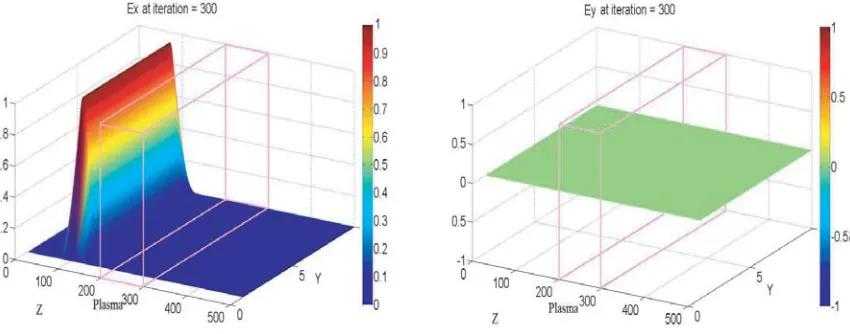
The electron collision frequency: ν_c = 2π × 3.18 ×109rad/s. The plasma frequency: ω_p = 2π ×50×109rad/s. The cyclotron frequency: ω_c = 2π×47.7×109rad/s. Generated in the tenths cells, the 2D electrical pulse used in this simulation is polarized in the X-direction and propagates in the positive Z-direction. Figure 1 illustrates the incident electric pulse after 300 iterations in the free space with the onlyE_x component. After penetration in the slab, E_y component appears changing to a negative value as shown in the 550th snapshot in Figure 2. In Figure 3, most of the incident wave crosses the medium, and a small portion is reflected to the first 200 cells region. Figure 4 demonstrates that transmitted and reflected components of the electric field are totally eliminated by an absorbing boundaries in the first and last cells according toZ-direction.

These figures illustrate the Faraday rotation effect in time domain. The initial plane of the linearly polarized wave is along X-direction. As the wave propagates through the gyroelectric medium, it starts to rotate in clockwise direction, and the wave can be regarded as a superposition of two circular polarization modes: Right-hand circular polarization (RCP) and Left-hand circular polarization (LCP). Electric field components are saved in one cell before and after the slab during 10000 iterations of the simulation then are transformed into frequency domain through fast Fourier transform. The reflection and transmission coefficients for right-hand circularly polarized (RCP) and left-hand circularly polarized (LCP) waves are calculated using:

Figure 1. Electric field components at the 300th iteration.

Figure 2. Electric field components at the 550th iteration.

Figure 3. Electric field components at the 750th iteration.

Figure 4. Electric field components at the 950th iteration.

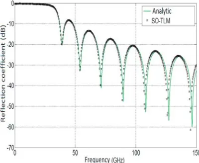
Figure 5. LCP reflection/transmission coefficient.

It can be observed that the SO-TLM curves are in excellent agreement with the exact analytical solution. Moreover, in Figure 6, SO-TLM result follows the exact transmission coefficient less than −180 dB which proves its efficiency.

3.2. Comparative Study

In this part, we will conduct a comparative study of the SO-TLM algorithm with five other techniques incorporated to the TLM method and presented in the literature: namely the method of the Constant Recursive Constant (CRC) [11], Piecewise Linear Recursive Convolution (PLRC) [12], Current Density Recursive Convolution (CDRC) also named (JEC) [5], Runge-Kutta Exponential Time Differencing (RKETD) [8], and Auxiliary Differential Equation (ADE) [9].

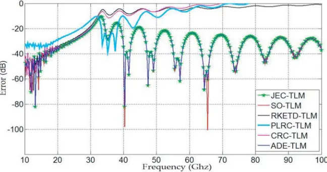
In order to obtain a classification that is independent of the physical performance of the computers or of a particular compiler, many criteria of algorithm complexity can be used. In the present study, we compare accuracies and execution time. In these numerical experiments, the same problem of Section3.1 has been taken up again and simulated by each approach. The calculation time is truncated after 3000 iterations. This can also give us an idea of the rate of convergence of each technique. Electrical field components have been recorded and are converted to the frequency domain using the Fourier transform. Then the coefficient of reflection of the resulting RCP wave is calculated by each algorithm. The relative error is defined as the difference between the analytic curve (reference) and the result of each algorithm, and is presented in a logarithmic scale in Figure 7.

Figure 7. Relative errors of different techniques in (dB).

The first remark that is obvious, which is that the error curves are divided into two groups: The first group, containing three curves at the top, is the least accurate. Indeed, it is clear that the RKETD-TLM approach is more accurate than PLRC-RKETD-TLM. However, the CRC is the worst technique in terms of accuracy. As for the accuracy of the second group’s algorithms, it is almost confused and still almost under 1%. We can finally offer a ranking of the approaches in the order of increasing precision as follows: CRC-TLM, PLRC-TLM, RKETD-TLM, (JEC-TLM and ADE-TLM are combined), while SO-TLM technique is the most accurate technique.

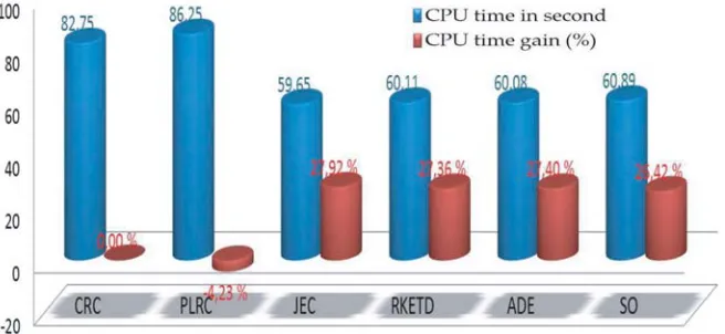
On the other hand, CPU time has been evaluated for each technique by considering a long slab of 800Δlof a magnetized plasma in the center of 1200Δlstructure. Each simulation lasts 15000 iterations. We measure the CPU time of each simulation and repeat the procedure ten times. In Figure 8, blue columns represent the average values of the CPU time. Since the CRC-TLM algorithm is more classic than the others, it has been considered as a reference algorithm. The latter lasts t_ref = 82.75 seconds. Then time gains are calculated as a percentage according to the equation:

CP UtimeGain=

1−ttechnique

Figure 8. RCP reflection/transmission coefficient.

We note that the execution time of the PLRC-TLM technique lasts t_{P LRC} = 86.25 seconds which presents a loss of time of 4.23%. The JEC-TLM, ADE-TLM, RKETD-TLM, and SO-TLM techniques represent a considerable gain of CPU time that exceeds 27%. According to Figure 8, different techniques rapidity ranking can be presented as follows: JEC, ADE, RKETD, SO, CRC, and PLRC.

The CRC-TLM, PLRC-TLM, RKETD-TLM, and JEC-TLM formulations are developed in a complex calculation that uses integrals and exponentials in the calculation of convolution products which are difficult to solve and also heavy to code. In addition, they are greedy in memory allocation. As for the two remaining techniques, SO-TLM and ADE-TLM, they are based respectively on the shift operator and Laplace transform. Their theoretical developments are relatively simple because they do not contain convolutions. They have a concise formulation and have the advantage of easily extensible beings in the most general cases of complex materials.

4. CONCLUSION

In this paper, we present a novel modeling approach to deal with gyroelectric media using the shift operator integrated in the TLM method. The high accuracy and efficiency of the proposed technique are verified by illustrating Faraday rotation in time domain and by calculating reflection and transmission coefficients through a gyroelectric slab. A comparison of SO-TLM with five other techniques from the literature demonstrate its competitivity.

REFERENCES

1. Paul, J., C. Christopoulos, and D. W. P. Thomas, “Generalized material models in TLM, I. Materials with frequency-dependent properties,” Transactions on Antennas and Propagation, Vol. 47, No. 10, 1528–1534, 1999.

2. Yagli, A. F., J. K. Lee, and E. Arvas, “Scattering from three-dimensional Dispersive Gyrotropic Bodies using the TLM method,”Progress In Electromagnetics Research B, Vol. 18, 225–241, 2003. 3. Yaich, M. I. and M. Khalladi, “An SCN-TLM model for the analysis of ferrite media,” IEEE

Microwave and Wireless Components Letters, Vol. 13, No. 6, 217–219, 2009.

4. Khalladi, M., M. I. Yaich, N. Aknine, and C. Carrion, “Modeling of electromagnetic waves propagation in non-linear optical media using HSCN-TLM method,” IEICE Electronics Express, Vol. 2, No. 13, 384–391, 2005.

6. Mounirh, K., S. El Adraoui, M. Charif, M. I. Yaich, and M. Khalladi, “Modeling of anisotropic magnetized plasma media using PLCDRC-TLM method,” International Journal for Light and Electron Optics, Vol. 126, No. 15–16, 1479–1482, 2015.

7. El Adraoui, S., A. Zugari, K. Mounirh, M. Charif, M. I. Yaich, and M. Khalladi, “Runge-Kutta exponential time differencing-TLM method for modeling cold plasma media,”International Conference on Multimedia Computing and Systems (ICMCS), 1363–1366, Marrakech, Morocco, 2014.

8. El Adraoui, S., M. Bassoh, M. Khalladi, M. I. Yaich, and A. Zugari, “RKETD-TLM modeling of anisotropic magnetized plasma,”International Journal of Science and Advanced Technology, Vol. 2, No. 8, 81–84, 2012.

9. Mounirh, K., S. El Adraoui, Y. Ekdiha, M. I. Yaich, and M. Khalladi, “Modeling of dispersive chiral media using the ADE-TLM method,” Progress In Electromagnetics Research M, Vol. 64, 157–166, 2018.

10. Attiya, A. M., “Shift-operator finite difference time domain analysis of chiral medium,” Progress In Electromagnetics Research M, Vol. 13, No. 10, 29–40, 2010.

11. Yaich, M. I., M. Khalladi, I. Zekik, and J. A. Morente, “Modeling of frequency-dependent magnetized plasma in hybrid symmetrical condensed TLM method,”IEEE Microwave and Wireless Components Letters, Vol. 12, No. 8, 193–195, 2002.

12. El Adraoui, S., A. Zugari, M. Bassouh, M. I. Yaich, and M. Khalladi, “Novel PLRC-TLM algorithm implementation for modeling electromagnetic wave propagation in gyromagnetic media,”