FRACTIONAL SURFACE WAVEGUIDE
H. Maab†
Ghulam Ishaq Khan Institute of Science and Technology Topi, Pakistan
Q. A. Naqvi
Department of Electronics Quaid-i-Azam University Islamabad, Pakistan
Abstract—Fractional curl operator has been utilized to study the fractional order surface waveguides. Fractional order surface waveguides may be regarded as intermediate step of two surface waveguides which are related through the principle of duality. Fractional eigenvalue equations are examined at the interface between dielectric medium and free space, for various values of fractional order parameter result in different fractional surface wave modes.
1. INTRODUCTION
Fractional curl operator which is represented ascurlα, whereαdenotes the order of the operator, obtains from fractionalization of the usual curl operator. Fractional curl operator constructs new set of solutions to Maxwell equations, which may be described as an intermediate steps between original solution set and the dual to the original solution set. These solutions are named as “fractional field” see for instance [1]. The applications of fractional curl operator was further extended by Naqvi et al. [2], they discussed the behavior of fractional dual solution in an unbounded chiral medium. Veliev and Engheta [3] and Ivakhnychenko et al. [4] utilized the fractional curl operator to a fixed solution and obtained the fractional fields that represent the solution of reflection problem from anisotropic surface impedance. Hussain and Naqvi [5], introduction the idea of fractional nonsymmetric transmission line.
Hussain et al. [6, 7], extended this idea to study fractional waveguides. Afterward Faryad and Naqvi [8] extended the work of fractional dual parallel plates waveguides and constructed the solutions corresponding to the fractional dual rectangular wave guides.
Propagation through waveguide structures has been studied by various authors [9–17]. In present paper we have extended the idea of fractional dual parallel plates waveguides [7] to surface waveguide or open waveguide. Surface waveguides are particularly used in millimetric-wave circuits. The fractional field expressions are carried out in both dielectric medium and free space. The fractional eigenvalue equations are examined numerically at the interface between dielectric medium and free space, taking t = λ0/4 and t = λ0/2, for
various values of fractional parameter α and results represent various intermediate fractional surface wave modes.
2. FRACTIONAL SURFACE WAVEGUIDE
Consider a surface waveguide composed of a dielectric of thickness “t” coated on plane perfect electric conductor. It is assumed to be of infinite extent in the y and z directions. We assume propagation in the +z direction with eiβz propagation factor and no variation in the y direction, that is (∂/∂y = 0). The geometry is divided into two regions. The first region (0< x < t) consists of dielectric material of permittivity = κ0 and the other region x > t represents the free space. The total TM fields for region 0< x < t may be written as
Ez = ˆzAsin(kdx) exp(iβz) (1a)
Ex = ˆx
iβ kd
Acos(kdx) exp(iβz) (1b)
ZHy = −yˆ
ik kd
Acos(kdx) exp(iβz) (1c)
where β2 = k2 − kd2, k = √κk0, k0 = ω√µ00, Z =
µ0
κ0, and
m−1
2 π ≤ kdt ≤
m
2π, m is positive integer. Z is the impedance of
the dielectric medium. For region t < x <∞
Ez = ˆzAsin(kdt) exp(−h(x−t) +iβz) (2a)
Ex = ˆx
iβ
hAsin(kdt) exp(−h(x−t) +iβz) (2b) Z0Hy = −yˆ
ik0
whereβ2 =k02−h2,Z0=µ0
0 implies thatkd=ihin free space, and
0< h <2n,nis positive integer.
We have first examined the fractional dual solutions of E-waves in the region 0< x < t. Total field in this region may be considered as combination of two TEM waves bouncing back and forth between the two boundaries, that is x = 0 and x = t. The x = 0 boundary represent PEC interface. For region 0< x < t, fields given in (1) may be written as
Ez = −izˆ
A
2[exp(ikdx+iβz)−exp(−ikdx+iβz)] (3a)
Ex = ˆx
iβ kd
A
2[exp(ikdx+iβz) + exp(−ikdx+iβz)] (3b)
ZHy = −yˆ
ik kd
A
2[exp(ikdx+iβz) + exp(−ikdx+iβz)] (3c) The total electric and magnetic fields in region 0< x < tare
E = E1+E2, (4a)
ZH = ZH1+ZH2 (4b)
where (E1,H1) represents the electric and magnetic fields related with
one plane wave and are given below
E1 = A
2
−izˆ+iβ
kd ˆ
x
exp(ikdx+iβz) (5a)
ZH1 = −A 2
k kd
iyˆexp(ikdx+iβz) (5b) The electric and magnetic fields related to other plane wave are represented by (E2,H2) as below
E2 = A
2
izˆ+ iβ
kd ˆ
x
exp(−ikdx+iβz) (6a)
ZH2 = − A
2
k kd
(ki×)α where i = 1,2. For this purpose, we need eigenvectors and eigenvalues of the (ki×), where ki are the wave vectors of the two plane wave bouncing back and forth. To determine the eigenvectors and eigenvalues of (k1×), we re-arrange Eq. (5) as follow
E1 = − Ak
2kd
izˆkd
k − iβ
kxˆ
exp(ikdx+iβz) (7a)
ZH1 = − Ak
2kd
iyˆexp(ikdx+iβz) (7b) The eigen vectors and eigen values of the operatork1×are
A1 =
1
√
2
−iβ
kxˆ+ ˆy+ ikd
k zˆ
, a1 =i A2 =
1
√
2
iβ
kxˆ+ ˆy− ikd
k zˆ
, a2 =−i A3 = −
ikd
k xˆ− iβ
kz,ˆ a3= 0
FieldE1 may be expressed in terms of the eigenvectors of k1×as
E1= [P1A1+Q1A2+R1A3] exp(ikdx+iβz) (8) where the coefficients are
P1 = − Ak
2√2kd
Q1 = Ak
2√2kd
R1 = 0
Using the fractional curl operator, fractional dual fields may be obtained using the following relations [2]
E1f d = [(ik)−1∇×]αE1 (9a)
ZH1f d = [(ik)−1∇×]α(ZH1) (9b)
It may be noted that |k1| = |k2|. This means that application of
fractional cross product operator (k1×)α on vectors (E1, ZH1) in
(ZH1,−E1) and are given as E1f d = (k1×)αE1
= −Ak 2kd
−iβ k cos απ 2 ˆ
x+isin απ
2
ˆ
y
+ikd
k cos απ 2 ˆ z
exp(ikdx+iβz) (10a)
ZH1f d = (k1×)αZH1
= −Ak 2kd
iβ k sin απ 2 ˆ
x+icos απ
2
ˆ
y
−ikd
k sin απ 2 ˆ z
exp(ikdx+iβz) (10b) The behavior of fractional electric and magnetic field represent a counterclockwise rotation by an angle απ/2.
To define the eigenvectors and eigenvalues of the cross product operator (k2×) Eq. (6) can be rearranged as follow
E2 = −kA 2kd
−ikd
k zˆ− iβ
kxˆ
exp(−ikdx+iβz) (11a)
ZH2 = − Ak
2kd
iyˆexp(−ikdx+iβz) (11b) Eigenvectors and eigenvalues of the operator (k2×) are
A1 =
1
√
2
−iβ
kxˆ+ ˆy− ikd
k zˆ
, a1 =i
A2 = √1 2
iβ
kxˆ+ ˆy+ ikd
k zˆ
, a2 =−i A3 = ikd
k xˆ− iβ
kz,ˆ a3 = 0
Vector E2 may be expressed as linear combination of eigenvectors of k2×
E2 = [P2A1+Q2A2+R2A3] exp(−ikdx+iβz) (12) where the coefficients are
P2 = − Ak
2√2kd
Q2 = Ak
2√2kd
The required fractional solutions of Eq. (12) may be considered as the intermediate step between the solution set (E2, ZH2) and the dual
solution set (ZH2,−E2) and are given by E2f d = (k2×)αE2
= −Ak 2kd
exp(−iαπ) −iβ k cos απ 2 ˆ
x−isin απ
2
ˆ
y
−ikd
k cos απ 2 ˆ z
exp(−ikdx+iβz) (13a)
ZH2f d = (k×)αZH1 = −Ak
2kd
exp(−iαπ) −iβ k sin απ 2 ˆ
x+icos απ
2
ˆ
y
−ikd
k sin απ 2 ˆ z
exp(−ikdx+iβz) (13b) If we summarize the fractional fields in the above equations, they show rotation by an angle of απ/2 in counterclockwise direction. Therefore the total fractional fields for the region 0 ≤ x ≤ t are considered to be the fractional intermediate steps between (E, ZH) and (ZH,−E). That shows rotation by an angle ofαπ/2 in counterclockwise direction. These are obtained by substituting the fractional results in Eq. (10) and Eq. (13) in Eq. (4)
Ef d=−
Ak kd
exp(−iαπ/2) −iβ k cos απ 2 cos
kdx+
απ 2 ˆ x −sin απ 2 sin
kdx+
απ
2
ˆ
y−kd kcos απ 2 sin
kdx+
απ 2 ˆ z
exp(iβz) (14a)
ZHf d=−
Ak kd
exp(−iαπ/2) −β ksin απ 2 sin
kdx+
απ
2
ˆ
x
+icos απ
2
cos
kdx+
απ
2
ˆ
y−ikd k sin απ 2 cos
kdx+
απ 2 ˆ z
exp(iβz) (14b)
To derive the fractional fields of the E-waves in free space x > t, rearrange Eq. (2)
E = −Ak0
h sin(kdt) exp(ht)
−iβ
k0xˆ− h k0zˆ
exp(−hx+iβz) (15a)
Z0H = − Ak0
The fractional dual fields in free space regionx > t become as follow
Ef d = −
Ak0
h sin(kdt)
−iβ k0 cos απ 2 ˆ x
+isin απ
2
ˆ
y− h k0 cos απ 2 ˆ z
exp(−h(x−t)+iβz) (16a)
Z0Hf d = −
Ak0
h sin(kdt)
iβ k0 sin απ 2 ˆ x
+icos απ
2
ˆ
y+ h
k0 sin απ 2 ˆ z
exp(−h(x−t)+iβz) (16b) For α = 0, we get the original solutions in both regions and for
α = 1 the fractional fields in both region rotated by an angle π/2 in counterclockwise direction, results in TE surface wave mode from TM surface wave mode.
The surface impedance of the fractional surface waves in dielectric region of thickness “t” obtained from Eq. (14a) and Eq. (14b) is
Zd=
Ezf d
Hyf d =ikd
kztan
kdx+
απ
2
(17)
and that in the free space (x > t) is
Zf ree =
Ezf d
Hyf d =ih
k0
z0 (18)
According to the transverse-resonance technique [9], the transverse resonance at x =t requires that the sum of impedances seen looking toward the shot-circuit(in this case the PEC atx= 0) and that at the input to the infinite line (in this casex > t) vanish. Therefore equating Eq. (17) and Eq. (18) gives the required fractional eigenvalue equation
ht= kdt
κ tan
kdt+
απ
2
(19)
where zk = z0
κk0. We note that for α= 0, Eq. (19) reduces to
ht= kdt
κ tan(kdt) (20)
which represent the eigenvalue equation of TM mode. But forα = 1, Eq. (19) gives the eigenvalue equation of TE mode that is
ht=−kdt
As the phase matching of tangential continuity at x = t interface for all value of zis achieved by the following relation
(kdt)2+ (ht)2 = (κ−1)(k0t)2 (22) which represents the equation of a circle of radius √κ−1(k0t).
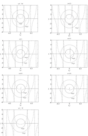
We have carried out the simultaneous numerical solution of Eq. (19) and Eq. (22) for t=λ0/4 and t=λ0/2, where λ0 is the free space wavelength, and κ = 2.56 as shown in Fig. 1. The two circles represented by solid line and dash line corresponded tot =λ0/4 and
t = λ0/2 respectively. For α = 0, circle corresponding to t = λ0/4 results in one TM surface wave mode, while circle for t=λ0/2 results
in two TM surface wave modes. We have obtained plots for various values of fractional parameter α. From the plots shown in Fig. 1, we have observed the following informations. For α = 0,0.25,0.5 or 0≤α ≤0.5, there exist one surface wave mode for t=λ0/4 and two
surface wave modes for t = λ0/2. But for α = 0.75,0.85,0.95,1 or
0.5≤α ≤1, we can see only one surface wave mode. This is because the TE mode in surface waveguide does not propagate until the radius of the circle,√κ−1(k0t), becomes greater thanπ/2 [18].
3. CONCLUSIONS
We have noted that for α = 0, we get the original TM fields in both dielectric and free space regions, but for α = 1, the electric and magnetic fields of original TM fields are rotated by an angle π/2 in counterclockwise direction and become TE surface wave modes. If the fractional fields are evaluated for higher order values of fractional parameter α, then for even values of α, we obtain TM surface wave modes and while for odd values of α we get TE surface wave modes. The corresponding fractional order surface wave eigen modes are analyzed for various values of α that show an intermediate steps between TM surface wave eigen modes and TE surface wave eigen modes.
REFERENCES
1. Engheta, N., “Fractional curl operator in electromagnetics,”
Microwave and Optical Technology Letters, Vol. 17, No. 2, 86–91, 1998.
2. Naqvi, Q. A., G. Murtaza, and A. A. Rizvi, “Fractional dual solutions to Maxwell equations in homogeneous chiral medium,”
3. Velied, E. I. and N. Engheta, “Fractional curl operator in reflection problems,” 10th Int. Conf. on Mathematical Methods in Electromagnetic Theory, Ukraine, Sept. 14–17, 2004.
4. Ivakhnychenko, M. V., E. I. Veliev, and T. M. Ahmedov, “Fractional operators approach in electromagnetic wave reflection problems,” Journal of Electromagnetic Waves and Applications, Vol. 21, No. 13, 1787–1802, 2007.
5. Hussain, A. and Q. A. Naqvi, “Fractional curl operator in chiral medium and fractional nonsymmetric transmission line,”Progress In Electromagnetics Research, Vol. 59, 119–213, 2006.
6. Hussain, A., S. Ishfaq, and Q. A. Naqvi, “Fractional curl operator and fractional waveguides,”Progress In Electromagnetics Research, PIER 63, 319–335, 2006.
7. Hussain, A., M. Faryad, and Q. A. Naqvi, “Fractional curl operator and fractional Chiro-waveguide,” Journal of Electromagnetic Waves and Applications, Vol. 21, No. 8, 1119– 1129, 2007.
8. Faryad, M. and Q. A. Naqvi, “Fractional rectangular waveguides,”
Progress In Electromagnetics Research, PIER 75, 383–396, 2007. 9. Rostami, A. and H. Motavali, “Asymptotic iteration method: A
powerful approach for analysis of inhomogeneous dielectric slab waveguides,” Progress In Electromagnetics Research B, Vol. 4, 171–182, 2008.
10. Cheng, Q. and T. J. Cui, “Guided modes and continuous modes in parallel-plate waveguides excited by a line source,”Journal of Electromagnetic Waves and Applications, Vol. 21, No. 12, 1577– 1587, 2007.
11. Li, Z., T. J. Cui, and J. F. Zhang, “TM wave coupling for high power generation and transmission in parallel-plate waveguide,”
Journal of Electromagnetic Waves and Applications, Vol. 21,
No. 7, 947–961, 2007.
12. Soekmadji, H., S.-L. Liao, and R. J. Vernon, “Trapped mode phenomena in a weakly overmoded waveguiding structure of rectangular cross section,”Journal of Electromagnetic Waves and Applications, Vol. 22, No. 1, 143–157, 2008.
13. Volski, V. and G. A. E. Vandenbosch, “Field generated by a magnetic line source embedded in a semi-infinite dielectric slab,”
Journal of Electromagnetic Waves and Applications, Vol. 19,
14. Dabirian, A. and M. Akbari, “Modal transmission-line theory of optical waveguides,” Journal of Electromagnetic Waves and Applications, Vol. 19, No. 7, 891–906, 2005.
15. Tomita, M. and Y. Karasawa, “Analysis of scattering and coupling problem of directional coupler for rectangular dielectric waveguides,”Journal of Electromagnetic Waves and Applications, Vol. 14, No. 9, 1261–1262, 2000.
16. Topa, A. L., C. R. Paiva, and A. M. Barbosa, “Complete spectral representation for the electromagnetic field of planar multi-layered waveguides containing pseudochiral O-media,”Journal of Electromagnetic Waves and Applications, Vol. 12, No. 3, 349–350, 1998.
17. Hayashi, Y., “Analysis of electromagnetic scattering by open boundary,” Journal of Electromagnetic Waves and Applications, Vol. 11, No. 6, 807–820, 1997.