ANALYSIS OF PLANAR MULTILAYER STRUCTURES AT OBLIQUE INCIDENCE USING AN EQUIVALENT BCITL MODEL
D. Torrungrueng and S. Lamultree
Department of Electrical and Electronic Engineering Faculty of Engineering and Technology
Asian University
Chon Buri, 20150, Thailand
Abstract—Planar multilayer structures have found several applica-tions in electromagnetics. In this paper, an equivalent model based on the bi-characteristic-impedance transmission line (BCITL) is employed to model planar multilayer structures effectively for bothlossless and
lossy cases. It is found that the equivalent BCITL model provides identical results, for both perpendicular and parallel polarizations, as those obtained from the propagation matrix approach.
1. INTRODUCTION
Multilayer structures have found several applications in electromagnet-ics; e.g., in the areas of optics, remote sensing and geophysics [1–13], especially for planar multilayer structures. Traditionally, the propa-gation matrix approach (PMA) is employed to solve problems related to planar multilayer structures rigorously [14]. Alternatively, it is well known that these problems can also be solved readily by modeling these structures using multi-section transmission lines with appropri-ate characteristic impedances and propagation constants, where each transmission line possesses the same length as of the corresponding layer [15, 16].
CCITLs cannot be used to modellossymulti-section transmission lines. Thus, one needs to resort to more general model for these cases.
In this paper, an equivalent model based on the bi-characteristic-impedance transmission line (BCITL) is employed to model planar multilayer structures effectively for both lossless and lossy cases. In general, BCITLs are lossy, and possess different characteristic impedancesZ0±b of wave propagating in opposite directions. Note that BCITLs can be practically implemented using finitelossy periodically loaded transmission lines, and a graphical tool, known asa generalized T-chart, has been recently developed for solving problems associated with BCITLs [19]. It should be pointed out that CCITLs are a special case of BCITLs when associated losses of BCITLs disappear and the passband operation is assumed.
This paper presents the propagation matrix approach in Section 2. Section 3 presents an equivalent model based on BCITLs. Then, numerical results of both approaches are compared in Section 4. Finally, conclusions are provided in Section 5.
2. PROPAGATION MATRIX APPROACH
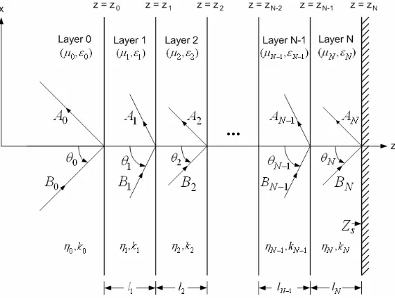
In this section, the propagation matrix approach is discussed for both perpendicular and parallel polarizations. Fig. 1shows a planar
multilayer structure terminated in a surface impedance ofZsatz=zN and illuminated by a plane wave of oblique incidence of the known amplitude B0 at the known incident angle θ0. Each layer of length li has the permeability µi, permittivityεi, intrinsic impedanceηi and wavenumberki, where i= 0, . . . , N. At each layer interface, Bi and Ai correspond to unknown amplitudes (B0 is known) of incident and reflected waves respectively, andθiis theunknown incident angle (θ0is known), which can be determined from the Snell’s law of refraction [14]. These wave amplitudes are associated with electric and magnetic fields for perpendicular and parallel polarizations, respectively. It should be pointed out thatµ0andε0are not necessarily the free space parameters in this notation.
Using the PMA [14], it is found that the wave amplitudes in Layers iand i+ 1are related by
Ai Bi
=[Li]
Ai+1 Bi+1
=1 2
(1+ri)ejkz,diffzi (1−ri)e−jkz,sumzi (1−ri)ejkz,sumzi (1+ri)e−jkz,diffzi
Ai+1 Bi+1
, (1)
where
kz,diff = kz, i+1−kz, i, (2)
kz,sum = kz, i+1+kz, i, (3)
kz, i = kicosθi, (4)
ri=
kz, i+1 kz, i
µi µi+1
, for perpendicular polarization
kz, i+1 kz, i
εi εi+1
, for parallel polarization.
. (5)
The total matrix [L] relating the wave amplitudes in Layers 0 and N is given in terms of the multiplication of each matrix [Li], where i= 0,1,2, . . . , N−1, as follows:
[L]=∆
L11 L12 L21 L22
= [L0][L1][L2]. . .[LN−2][LN−1]. (6)
Once the matrix [L] is computed by using Eqs. (1) and (6), the total input reflection coefficient Γ0, defined at the interface between Layers 0 and 1, can be determined in terms of each element of [L] as
Γ0 ∆ = A0
B0
= L11RNe−
j2kz, NzN+L
12 L21RNe−j2kz, NzN+L22
where
RN =
kz, NZs−ωµN kz, NZs+ωµN
, for perpendicular polarization
kz, NYs−ωεN kz, NYs+ωεN
, for parallel polarization
, (8)
and Ys = Zs−1 is the surface admittance at z = zN. In the next section, the equivalent model based on BCITLs is developed for planar multilayer structures.
3. EQUIVALENT MODEL BASED ON BCITLS
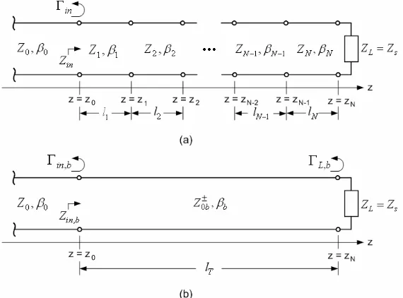
As pointed out earlier, planar multilayer structures can be analyzed by modeling these structures using multi-section transmission lines. Fig. 2(a) illustrates the equivalent multi-section model of Fig. 1, where the propagation constant βi and the characteristic impedance Zi of each transmission line in the multi-section model are defined as
βi =kz, i, (9)
Zi=
ηisecθi, for perpendicular polarization
ηicosθi, for parallel polarization . (10)
The multi-section model can be analyzed effectively using the BCITL model shown in Fig. 2(b). In [17] and [20], the characteristic impedances Z0±b and the propagation constant βb can be determined from the total transmission (ABCD) matrix of thecascading N-section transmission lines of the total lengthlT in Fig. 2(a) as
Z0±b = ∓2B
(A−D)∓j4−(A+D)2 (11)
cos (βblT) =
A+D
2 . (12)
Note that the formula of the ABCD matrix of each N-section transmission line is provided in [20].
Figure 2. Transmission line models: (a) Multi-section model and (b) BCITL model.
z = z0 and z = zN respectively as shown in Fig. 2. This is due to the fact that the multi-section transmission line in Fig. 2(a) is globally viewed as a two-port network in constructing the BCITL model.
The total input reflection coefficient Γin, b in Fig. 2(b) can be determined from the input impedanceZin, b as
Γin, b=±
Zin, b−Z0 Zin, b+Z0
, (13)
where
Zin, b = Z0+bZ0−b
1 + ΓL, be−j2βblT Z0−b−Z0+bΓL, be−j2βblT
(14)
ΓL, b =
ZsZ0−b−Z + 0bZ0−b
ZsZ0+b+Z0+bZ0−b. (15)
The derivation of Zin,b and ΓL, b can be found in [21]. Note that the load reflection coefficient ΓL, b associated with the BCITL is defined at z = zN. In Eq. (13), the plus and minus signs correspond to the perpendicular and parallel polarizations, respectively. The minus
associated with the current, instead of the voltage, for the parallel polarization. In the next section, numerical results of both approaches are compared.
4. NUMERICAL RESULTS
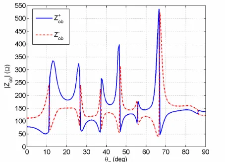
For illustration of the validity of the equivalent BCITL model, consider a lossy planar three-layer structure (N = 3) illuminated by an oblique plane wave at 18 GHz and terminated in a surface impedance of Zs = 50.0 Ω. Parameters of each layer are given as follows: µr,0 = µr,1 = µr,2 = µr,3 = 1.0, εr,0 = 1.0, εr,1 = 5.0 −j0.01, εr,2 = 1 0.0−j0.05, εr,3 = 1 4.0−j0.01, z0 = 0.0 m, z1 = 0.1 0 m, z2 = 0.15 m andz3= 0.30 m.
For the perpendicular polarization, Figs. 3 and 4 illustrate the plots of the magnitude and phase of the characteristic impedancesZ0±b computed by using Eq. (11) versus the incident angle θ0, respectively. Note that Z0+b and Z0−b are generally complex and different. These results are consistent with the fact that the structure of interest is
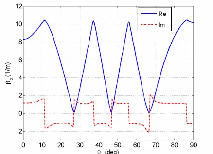
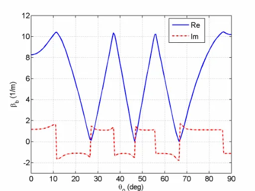
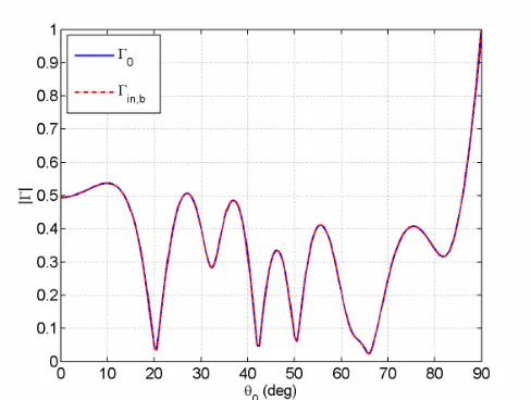
lossy. In addition, Z0±b vary considerably with θ0. Fig. 5 shows the plot of the real and imaginary parts of the propagation constant βb versus θ0. Note that βb is also complex in general due to the lossy structure of interest, and it varies noticeably withθ0. Fig. 6 shows the plot of the magnitude of the total input reflection coefficient versusθ0 for both PMA (Γ0) and equivalent BCITL model (Γin, b). It is obvious that numerical results obtained from both approaches are identical for
Figure 4. Plot of the phase of the characteristic impedances Z0±b versusθ0 for the perpendicular polarization.
Figure 5. Plot of the real and imaginary parts of the propagation constantβb versusθ0 for the perpendicular polarization.
all θ0 of interest.
Figure 6. Plot of the magnitude of the total input reflection coefficient versusθ0 for the perpendicular polarization.
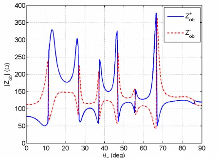
Figure 7. Plot of the magnitude of the characteristic impedancesZ0±b versusθ0 for the parallel polarization.
Figure 8. Plot of the phase of the characteristic impedances Z0±b versusθ0 for the parallel polarization.
Figure 10. Plot of the magnitude of the total input reflection coefficient versus θ0 for the parallel polarization.
5. CONCLUSIONS
Planar multilayer structures at oblique incidence can be analyzed successfully using an equivalent BCITL model for both perpendicular and parallel polarizations. The variations of BCITL parameters, Z0±b andβb, with the incident angleθ0 are studied as well. It is found that these parameters are generally complex and strongly dependent on θ0 for both polarizations. In addition, the magnitude of the total input reflection coefficient obtained from both PMA and equivalent BCITL model are identical indeed. Finally, the equivalent BCITL model is conceptually simple and effective, and may offer better physical insight into more complicated multilayer structures.
REFERENCES
1. Qing, A. and C. K. Lee, “An improved model for full wave analysis of multilayered frequency selective surface with gridded square element,” Progress In Electromagnetics Research, PIER 30, 285– 303, 2001.
2. Kong, J. A., “Electromagnetic wave interaction with stratified negative isotropic media,”Progress In Electromagnetics Research, PIER 35, 1–52, 2002.
planar layers using Taylor’s series expansion,” IEEE Trans. Antennas and Propagation, Vol. 54, No. 1, 130–135, Jan. 2006. 4. Khalaj-Amirhosseini, M., “Analysis of lossy inhomogeneous
planar layers using finite difference method,” Progress In Electromagnetics Research, PIER 59, 187–198, 2006.
5. Rothwell, E. J., “Natural-mode representation for the field reflected by an inhomogeneous conductor-backed material layer – TE case,”Progress In Electromagnetics Research, PIER 63, 1–20, 2006.
6. Kedar, A. and U. K. Revankar, “Parametric study of flat sandwich multilayer Radome,” Progress In Electromagnetics Research, PIER 66, 253–265, 2006.
7. Aissaoui, M., J. Zaghdoudi, M. Kanzari, and B. Rezig, “Optical properties of the quasi-periodic one-dimentional generalized multilayer fibonacci structures,” Progress In Electromagnetics Research, PIER 59, 69–83, 2006.
8. Khalaj-Amirhosseini, M., “Analysis of lossy inhomogeneous planar layers using equivalent sources method,” Progress In Electromagnetics Research, PIER 72, 61–73, 2007.
9. Khalaj-Amirhosseini, M., “Analysis of lossy inhomogeneous planar layers using the method of moments,” Journal of Electromagnetic Waves and Applications, Vol. 21, No. 14, 1925– 1937, 2007.
10. Khalaj-Amirhosseini, M., “Analysis of lossy inhomogeneous planar layers using fourier series expansion,” IEEE Trans. Antennas and Propagation, Vol. 55, No. 2, 489–493, Feb. 2007. 11. Suyama, T., Y. Okuno, A. Matsushima, and M. Ohtsu, “A
numer-ical analysis of stop band characteristics by multilayered dielectric gratings with sinusoidal profile,”Progress In Electromagnetics Re-search B, Vol. 2, 83–102, 2008.
12. Yildiz, C. and M. Turkmen, “Quasi-static models based on artificial neural neworks for calculating the characteristic parameters of multilayer cylindrical coplanar waveguide and strip line,”Progress In Electromagnetics Research B, Vol. 3, 1–22, 2008. 13. Oraizi, H. and A. Abdolali, “Combination of MLS, GA & CG for the reduction of RCS of multilayered cylindrical structures composed of dispersive metamaterials,” Progress In Electromagnetics Research B, Vol. 3, 227–253, 2008.
14. Kong, J. A., Electromagnetic Wave Theory, 2nd edition, Wiley-Interscience, NY, 1990.
Sigapore, 1989.
16. Oraizi, H. and M. Afsahi, “Analysis of planer dielectric multilayers as FSS by transmission line transfer matrix method (TLTMM),”
Progress In Electromagnetics Research, PIER 74, 217–240, 2007. 17. Worasawate, D. and D. Torrungrueng, “Analysis of a multi-section
impedance transformer using an equivalent CCITL model,”Proc. of the 2006 ECTI-CON, 111–114, Ubon Ratchatani, Thailand, May 10–13, 2006.
18. Torrungrueng, D., C. Thimaporn, and N. Chamnandechakun, “An application of the T-chart for solving problems associated with terminated finite lossless periodic structures,”Microwave and Optical Tech.Lett., Vol. 47, No. 6, 594–597, December 2005. 19. Torrungrueng, D., P. Y. Chou, and M. Krairiksh, “A graphical
tool for analysis and design of bi-characteristic-impedance transmission lines,” Microwave and Optical Tech.Lett., Vol. 49, No. 10, 2368–2372, October 2007.
20. Pozar, D. M., Microwave Engineering, 3rd edition, Wiley, NJ, 2005.