ABSTRACT
PAYNE, MATTHEW JORDAN. Three-Dimensional Microphysical and Dynamical Structures of Winter Storms in the U.S. Pacific Northwest. (Under the direction of Sandra Yuter).
Frequent rainfall during the winter months in the Portland, Oregon region is associated with extratropical cyclones modified by the Coastal and Cascade Ranges. Operational WSR-88D radar observations from Portland, OR and upper-air soundings from Salem, OR over a 3-year period (2003-2006) from 1 November – 31 March are used to determine a 3D climatology of winter storms. 84 % of the 117 storm events had a low-level wind direction from the south or southwest, between 158° - 248° azimuth. Stability varied between storms, with most storms being neutral to slightly stable. Wind direction was found to be more important in determining the geographic pattern of precipitation in the PNW. For S-SW flow storms, increasing the storm volume is primarily related to increasing precipitation frequency rather than precipitation areal coverage. Local maximum in precipitation frequency is seen
typically at mid-windward slope rather than at the Cascade Range crest. 3D radar observations were also compared to MM5 output for the 2005-06 and 2006-07 winter seasons. Storms were grouped by their prevailing low-level wind direction and two individual cases (2005 Dec 29-31; 2006 Nov 6-7) to compare their radial velocity,
Three-Dimensional Microphysical and Dynamical Structures of Winter Storms in the U.S. Pacific Northwest
by
Matthew Jordan Payne
A thesis submitted to the Graduate Faculty of North Carolina State University
in partial fulfillment of the requirements for the Degree of
Master of Science
Marine, Earth, and Atmospheric Sciences
Raleigh, North Carolina
2007
APPROVED BY:
_____________________ __________________________ Dr. William Showers Dr. Sankar Arumugam
________________________________ Dr. Sandra Yuter
DEDICATION
To my wonderful parents, Matthew Dunn Payne and Tammy Winstead Payne for being the
best parents two sons could ever have, and for giving every ounce of resource and energy to
making my brother, Michael Dunn Payne, and I successful. To the rest of my family for
being there throughout the good and bad times, and for the wonderful support I had while in
graduate school. Also, to my wonderful friends who have helped me through times a grief
and have always been there for me.
ACKNOWLEDGEMENTS
I sincerely thank Dr. Sandra Yuter for providing me this wonderful opportunity to
research this topic on orographic precipitation. I would also like to thank my committee
members Dr. William Showers and Dr. Sankar Arumugam for providing advice and input
into my thesis paper and defense. Greatly appreciated are the model output and advice from
collaborators Dr. Brian Colle and Yanluan Lin of Stony Brook University. They provided
MM5 output, Hovmoeller plots of radar data, and analysis of storm over, under and good
prediction based on comparison of model output to SNOTEL data. Special thanks to
Catherine Spooner, Kimberly Comstock, and Tim Downing for advice and technical help.
Also, additional thanks go to David Stark for supplying the MRR plots and Diana Thomas
for ESRL Reanalysis figures. Funding was provided by the National Science Foundation
grants ATM-0544766 (Yuter) and ATM-0450444 (Colle).
TABLE OF CONTENTS
List of Figures --- v
Chapter 1. Introduction --- 1
Chapter 2. Data and Methods --- 7
2.1 Radar data --- 8
2.2 Radar mean, standard deviation, and precipitation frequency --- 9
2.4 Upper-air sounding data --- 10
2.5 Willamette Valley airflow characteristics --- 11
Chapter 3. Radar Climatology Results --- 14
3.1 Low-level wind direction --- 14
3.2 Cross-barrier wind speed --- 17
3.3 Brunt-Väisälä frequency --- 19
3.4 Time-accumulated precipitation volume --- 20
Chapter 4. Radar & Model Data Comparison Results --- 22
4.1 Storm-averaged radial velocity --- 24
4.1.1 SE storms --- 24
4.1.2 S-SW storms --- 25
4.1.3 W-NW storms --- 26
4.2 Precipitation Frequency --- 27
4.2.1 SE storms --- 27
4.2.2 S-SW storms --- 28
4.2.3 W-NW storms --- 28
4.3 2005 December 29 – 31 storm --- 29
4.3.1 Mean and standard deviation of radial velocity--- 30
4.3.2 Precipitation frequency --- 31
4.4 2006 November 6 – 7 storm --- 32
4.4.1 Mean and standard deviation of radial velocity --- 34
4.4.2 Precipitation frequency --- 35
Chapter 5. Discussion --- 35
5.1 James and Houze (2005) --- 35
5.2 Medina and Houze (2003) --- 36
5.3 Medina et al. (2007) --- 37
Chapter 6. Conclusions --- 39
References --- 95
LIST OF FIGURES
Chapter 1. Introduction
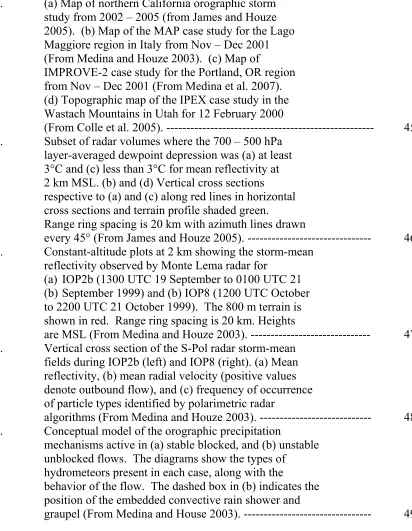
Fig. 1. (a) Map of northern California orographic storm study from 2002 – 2005 (from James and Houze 2005). (b) Map of the MAP case study for the Lago Maggiore region in Italy from Nov – Dec 2001 (From Medina and Houze 2003). (c) Map of
IMPROVE-2 case study for the Portland, OR region from Nov – Dec 2001 (From Medina et al. 2007). (d) Topographic map of the IPEX case study in the Wastach Mountains in Utah for 12 February 2000
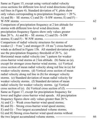
(From Colle et al. 2005). --- 45 Fig. 2. Subset of radar volumes where the 700 – 500 hPa
layer-averaged dewpoint depression was (a) at least 3°C and (c) less than 3°C for mean reflectivity at 2 km MSL. (b) and (d) Vertical cross sections respective to (a) and (c) along red lines in horizontal cross sections and terrain profile shaded green. Range ring spacing is 20 km with azimuth lines drawn
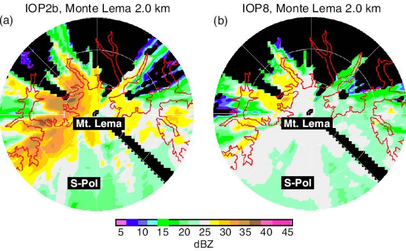
every 45° (From James and Houze 2005). --- 46 Fig. 3. Constant-altitude plots at 2 km showing the storm-mean
reflectivity observed by Monte Lema radar for
(a) IOP2b (1300 UTC 19 September to 0100 UTC 21 (b) September 1999) and (b) IOP8 (1200 UTC October to 2200 UTC 21 October 1999). The 800 m terrain is shown in red. Range ring spacing is 20 km. Heights
are MSL (From Medina and Houze 2003). --- 47 Fig. 4. Vertical cross section of the S-Pol radar storm-mean
fields during IOP2b (left) and IOP8 (right). (a) Mean reflectivity, (b) mean radial velocity (positive values denote outbound flow), and (c) frequency of occurrence of particle types identified by polarimetric radar
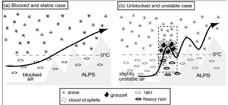
algorithms (From Medina and Houze 2003). --- 48 Fig. 5. Conceptual model of the orographic precipitation
mechanisms active in (a) stable blocked, and (b) unstable unblocked flows. The diagrams show the types of
hydrometeors present in each case, along with the
behavior of the flow. The dashed box in (b) indicates the position of the embedded convective rain shower and
graupel (From Medina and House 2003). --- 49
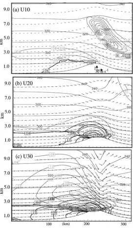
Fig. 6. Idealized 2-D cross section of potential temperature (solid every 10 K), wind vectors, snow (gray-dashed), graupel (black-dashed), and rain (solid) mixing ratios every 0.08 g kg−1 starting at 0.04 g kg−1 for the cases of increasing wind speed perpendicular to the mountain for (a) cross-barrier wind speed at 10 ms-1 (U10), (b) cross-barrier wind speed at 20ms-1 (U20), and (c) cross-barrier wind
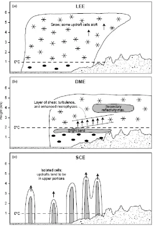
speed at 30 ms-1 (U30) experiments (From Colle 2004). --- 50 Fig. 7. Schematic illustration of the typical reflectivity structures
observed in the (a) Leading Edge Echo, (b) Double Maximum Echo, and (c) Shallow Convective Echo periods of
mid-latitude Pacific cyclones as they progress toward the terrain of the Oregon Cascade Range. The solid contours enclose areas of moderate reflectivity, while the shading indicates areas of increased reflectivity. The stars indicate snow and the ellipses rain. The speckled area shows the orography. The arrow represents updrafts (From
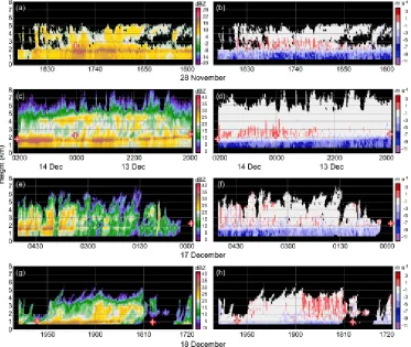
Medina et al. 2007). --- 51 Fig. 8. Time series of S-band vertically pointing profiler radar
(S-Prof) data during the passage of double maximum echo periods for reflectivity (left) and radial velocity (right): (a)-(b) 1600-1900 UTC 28 November 2001; (c)-(d) 2000 UTC 13 December – 0200 UTC 14 December 2001; (e)-(f) 0000-0500 UTC 17 December 2001; and (g)-(h) 1720-2000 UTC 18 December 2001. The crosses show the height of the 0° C level as measured by the Salem soundings. Note only storm in (c) shows distinct double maximum echo
(From Medina et al. 2007). --- 52 Fig. 9. Comparison of observed model variables for IPEX case.
(a) Plots of liquid water mixing ratio (g kg-3) from the King Probe (dashed) and 1.33-km MM5 (solid) at 4356, 3756, 3110, and 2812 m MSL. (b) Plots of snow mixing ratio (g kg−1) derived from the composite 2DGC–2DP particle size spectra (gray dashed) and 1.33-km MM5 (black) at 4356, 3756, 3110, and 2812 m MSL. The location of the crest is shown by the gray vertical line
(From Colle et al. 2005a). --- 53 Fig. 10. Sea surface temperatures that show the typical atmospheric
responses to shifts the ocean temperature during (a) El Nino and (b) La Nina (Taylor 1998). (c) Pacific Decadal
Oscillation (PDO) monthly index from 1900 through
Feb. 2007 (JISAO). --- 54
Chapter 2. Data and Methods
Fig. 11. (a) Average annual precipitation (in inches) for thirty-year (1961 – 1990) climatology of the U.S. Pacific Northwest. The diagram shows enhanced precipitation associated with Coastal (left side) and Cascade (right side) Ranges in the analysis area (From Daly et al. 1994). (b) Topography of Portland, Oregon and its surrounding areas (in km altitude). Locations of Coastal and Cascade Ranges, Portland
NEXRAD radar (circle), Salem sounding (triangle), and
Willamette Valley are labeled. --- 55 Fig. 12. Precipitation frequency (%) plots and standard deviation of
radial velocity for S-SW storms for all three winter seasons. (a),(c) represent unmasked precipitation frequency for S-SW storms. (b),(d) represent masked precipitation frequency (≤ 20 %) for S-SW storms. (e),(g) Unmasked standard deviation of radial velocity for S-SW storms. (f),(h) Masked
standard deviation of radial velocity for S-SW storms. --- 56 Fig. 13. (a) Histogram of vertically averaged wind direction storms
for 117 storms over three winter seasons. Storms are separated by wind directions (black line); A – SE storms (9 total), B – S-SW storms (98), and C – W-NW storms (10) for averaged plots in Figs. 15 – 17. (b) Scatter plot of vertically averaged cross-barrier wind speed versus wind direction for layer (0.61 - 2.2 km altitude) from Salem (SLE) upper-air soundings. Box shows categories of weak wind speed (2 - 9 ms-1) and stronger wind speed (9 - 18 ms-1) storms for those with 180º - 260º azimuth layer-averaged wind direction for averaged plots in Figs. 18 – 19. (c) Scatter plot of vertically averaged moist squared Brunt-Väisälä frequency (s-1) versus wind direction for layer (0.61 - 2.2 km altitude). Black line indicates separation of unstable (B-V < 0) and stable/neutral (B-V ≥ 0) storms used for averaged plots in Figs. 20 – 21. (d) Similar plot as (c) except B-V versus cross-barrier wind speed (ms-1). (e) Scatter plot of Froude number versus wind speed (ms-1) using the 800 – 900 hPa
layer average. --- 58
Fig. 14. (a) Scatter plot of storm total precipitation volume (Z ≥ 13 dBZ) versus Froude number for 800 – 900 hPa layer for all 117 storms. (b) Same as (a), except for vertically averaged wind direction using 0.61 – 2.2 km layer average. Green line represents threshold of 2 x 10⁷ km3 as separation between large and small storms for Figs. 22 and 23. (c) Same as (b), except for Brunt-Väisälä frequency (s-1). Black lines indicated threshold of 2 x 10⁷ km3 for storm total accumulated volumes and 0 s-2 for stability. (d) Same as (b), except for vertically averaged total wind speed. (e) Same as (b), except for vertically averaged cross-barrier wind speed (ms-1). Black line indicates separation at 9ms-1 for weak (U < 9ms-1) and strong ( U ≥ 9ms-1) cross-barrier wind speed storms. (f) Histogram of storm total accumulated volumes of precipitation frequency (Z ≥ 13 dBZ) for 117 storms over
three winter seasons. --- 59
Chapter 3. Radar Climatology Results
Fig. 15. Comparison of radial velocity structures (at 2 km altitude) for storms with different low-level wind directions (from Figure 13a). All Vr standard deviation figures show only values correspond to points with precipitation frequency > 20 %. (a) Horizontal mean radial velocity pattern for SE storms. (b) Horizontal standard deviation of mean radial velocity for (a). (c) Same as (a) except for S-SW storms. (c) Horizontal standard deviation of mean radial velocity for (c). (e) Same as (a) and (b) except for W-NW storms. (f) Horizontal standard deviation of mean radial velocity for (e). Comparison of horizontal radial velocity structures (at 1 km altitude) for storms with different low-level wind directions as defined in Figure 13a. Standard deviation of Vr plots show only values corresponding to precipitation frequency > 20 %. (g) Horizontal mean radial velocity pattern for SE storms. (h) Horizontal standard deviation of mean radial velocity for (g). (i) Same as (g) except for S-SW storms. (j) Horizontal standard deviation of mean radial velocity for (i). (k) Same as (g) and (i) except for W-NW storms. (l) Horizontal standard deviation of mean
radial velocity for (k). --- 60
Fig. 16. Same as Figure 15, except using vertical radial velocity cross sections for different low-level wind directions (along red lines in Figure 4). Standard deviation of Vr plots show only values corresponding to precipitation frequency > 20 %. A) and B) - SE storms; C) and D) - S-SW storms; E) and F) –
W-NW storms. --- 62 Fig. 17. Comparison of precipitation frequency at 2 km altitude for
storms with different low-level wind directions. All precipitation frequency figures show only values greater than 20 %. A) and B) - SE storms; C) and D) - S-SW
storms; E) and F) - W-NW storms. --- 63 Fig. 18. Comparison of radial velocity structures for storms of
weaker (2 – 9 ms-1) and stronger (9 -18 ms-1) cross-barrier winds as defined in Figure 13b. All standard deviation plots use the precipitation frequency threshold of 20 %. (a) Horizontal mean radial velocity (ms-1) pattern for weaker cross-barrier wind storms at 2 km altitude. (b) Same as (a), except for stronger cross-barrier wind storms. (c) Vertical cross section of mean radial velocity along red line in (a) for weaker velocity storms. (d) Vertical cross section of mean radial velocity along red line in (b) for stronger velocity storms. (e) Standard deviation of mean radial velocity for weaker velocity storms. (f) Standard deviation of mean radial velocity for weaker velocity storms. (g) Vertical
cross section of (e). (h) Vertical cross section of (f). --- 64 Fig. 19. Same as Figure 17, except for precipitation frequency for
lower and higher cross-barrier wind speeds. All precipitation frequency figures show only values greater than 20 %. A) and C) – Weak cross-barrier wind speed storms; B) and D) – Strong cross-barrier wind speed storms; E) and G) – Two largest accumulated volume storms; G) and H) Strong cross-barrier wind speed storms without
the two largest accumulated volume storms. --- 66
Fig. 20. Comparison of radial velocity structures for storms with unstable (B-V < 0 s-1) and stable (0.15 x 10⁻⁴ s-1 < B-V < 4 x 10⁻⁴ s-1) storms as defined in Figure 13c. All standard deviation plots use the precipitation frequency threshold > 20 %. (a) Horizontal mean radial velocity (ms-1) pattern for unstable storms at 2 km altitude. (b) Same as (a), except for stable storms. (c) Vertical cross section of mean radial velocity along red line in (a) for unstable storms. (d) Vertical cross section of mean radial velocity along red line in (b) for stable storms. (e) Standard deviation of mean radial velocity for unstable storms. (f) Standard deviation of mean radial velocity for stable storms. (g) Vertical cross section of (e).
(h) Vertical cross section of (f). --- 68 Fig. 21. Same as Figure 19, except for precipitation frequency for
unstable and stable storms. All precipitation frequency figures show only values greater than 20 %. A) and C) – unstable
storms; B) and D) – stable storms. --- 70 Fig. 22. Comparison of radial velocity structures for storms for
large (volume > 2 x 10⁷ km3) and small (volume < 2 x 10⁷ km3) volume storms as defined in Figure 14a. All standard deviation plots use the precipitation frequency threshold > 20 % (a) Horizontal mean radial velocity (ms-1) pattern for large storms at 2 km level. (b) Same as (a), except for small storms. (c) Vertical cross section of mean radial velocity along red line in (a) for large storms. (d) Vertical cross section of mean radial velocity along red line in (b) for small storms. (e) Standard deviation of mean radial velocity for large storms. (f) Standard deviation of mean radial velocity for small storms. (g) Vertical cross section
of (e). (h) Vertical cross section of (f). --- 71 Fig. 23. Same as Figure 21, except for precipitation frequency for
large and small volume storms. All precipitation frequency figures show only values greater than 20 %. A) and C) – large
volume storms; B) and D) – small volume storms. --- 73 Fig. 24. Time versus distance plots along E-W line at 45.35° N
latitude for (a) 2005 Nov 4 (small volume storm) and (b) 2005 Dec 30 (large volume storm) (Yanluan Lin, personal communication). (c) Time (UTC) versus distance diagram of Monte Lema radar reflectivity along 9.15°E at 4 km altitude for 20 September 1999. Measurements are every 7.5 minutes. Orographic precipitation locked to the terrain
(From Smith et al. 2003). --- 74
Chapter 4. Radar & Model Data Comparison Results
Fig. 25. (a) Moist Squared Brunt-Väisälä Frequency (s-2) versus layer-averaged wind direction for all SNOTEL storms (57) during the 2005-2006 winter season. (b) Scatter plot of storm total precipitation volume (Z ≥ 13 dBZ) versus vertically averaged cross-barrier wind speed (ms-1). (c) Scatter plot of storm total precipitation volume (Z ≥ 13 dBZ) versus vertically averaged wind speed (ms-1). Analysis of good, under, and over prediction cases by Yanluan Lin of Stony Brook University based on SNOTEL snow gauge stations in the
Western U.S. --- 75 Fig. 26. Comparison of radial velocity structures (ms-1) for
southeasterly (SE) storms for the 2005-2006 winter storm season. Observed standard deviation plots use the precipitation frequency threshold > 20 %. (a) Horizontal mean radial velocity pattern for observed SE storms. (b) Same as (a) except for
model SE storms. (c) Vertical cross section along red line in (a). (d) Vertical cross section along red line in (b). (e) Standard deviation values of (a). (f) Standard deviation values of (b). (g) Vertical cross section along red line in (e). (h) Vertical cross
section along red line in (f). --- 76 Fig. 27. Comparison of radial velocity structures (ms-1) for
south/southwest (S-SW) storms for the 2005-2006 winter storm season. Observed standard deviation plots use the precipitation frequency threshold > 20 %. (a) Horizontal mean radial velocity pattern for observed S-SW storms. (b) Same as (a) except for model S-SW storms. (c) Vertical cross section along red line in (a). (d) Vertical cross section along red line in (b). (e) Standard deviation values of (a). (f) Standard deviation values of (b). (g) Vertical cross section along red line in (e). (h)
Vertical cross section along red line in (f). --- 78 Fig. 28. Comparison of radial velocity structures (ms-1) for
west/northwest (W-NW) storms for the 2005-2006 winter storm season. Observed standard deviation plots use the precipitation frequency threshold > 20 %. (a) Horizontal mean radial velocity pattern for observed W-NW storms. (b) Same as (a) except for model W-NW storms. (c) Vertical cross section along red line in (a). (d) Vertical cross section along red line in (b). (e) Standard deviation values of (a). (f) Standard deviation values of (b). (g) Vertical cross section along red
line in (e). (h) Vertical cross section along red line in (f). --- 80
Fig. 29. Comparison of precipitation structures for southeast (SE) storms for the 2005-2006 winter storm season. Radar
observations are on the left, while model output is to the right. Observed precipitation frequency figures show only values > 20 %. (a) Horizontal precipitation frequency (%) pattern for observed SE storms. (b) Same as (a) except for model SE storms. (c) Vertical cross section along red line from (a). (e) Vertical cross section along red line in (b) with QT frequency as contours and potential temperature as filled
contours. --- 82 Fig. 30. Comparison of precipitation structures for south/southwest
(S-SW) storms for the 2005-2006 winter storm season. Radar observations are on the left, while model output is to the right. Observed precipitation frequency figures show only values > 20 %. (a) Horizontal precipitation frequency (%) pattern for observed S-SW storms. (b) Same as (a) except for model S-SW storms. (c) Vertical cross section along red line from (a). (d) Vertical cross section along red line in (b) with QT frequency as contours and potential
temperature as filled contours. --- 83 Fig. 31. Comparison of precipitation structures for west/northwest
(W-NW) storms for the 2005-2006 winter storm season. Radar observations are on the left, while model output is to the right. Observed precipitation frequency figures show only values > 20 %. (a) Horizontal precipitation frequency (%) pattern for observed W-NW storms. (b) Same as (a) except for model W-NW storms. (c) Vertical cross section along red line from (a). (d) Vertical cross section along red line in (b) with QT frequency as contours and potential
temperature as filled contours. --- 84 Fig. 32. Characteristics of the 2005 December 29 – 31 storm. (a)
Reanalysis plot of surface pressure (hPa) for 24-h period on 2005 Dec 30 (ESRL Reanalysis). (b) Reanalysis plot of precipitable water (mm) for 24-h period on 2005 Dec 30 (ESRL Reanalysis). (c) Total hourly precipitation (mm) from PDX for 2100 UTC 29 Dec 2005 to 0400 UTC 31 Dec 2005. (d) Hourly surface pressure (hPa) for same time period as (c). (e) Hourly surface temperature (° C) for same time period as (c). (f) Hourly wind direction (deg azimuth)
for same time period as (c). --- 85
Fig. 33. (a) Vertical profile of SLE sounding for 1200 UTC 30 Dec 2005 representative of flow during the 2005 Dec 29-31 storm. (b) Time height plot of Micro Rain Radar (MRR) vertically pointing radar data for Portland, OR during the 2005 Dec 29-31 storm. Period begins after 1600 UTC 30 Dec 2005 due
to missing data. --- 86 Fig. 34. Comparison of radial velocity structures (ms-1) for the 2005
December 29-31 storm case. Radar observations are on the left, while model output is to the right. Observed precipitation frequency figures show only values > 20 %. (a) Horizontal mean radial velocity pattern for observed SE storms. (b) Same as (a) except for model SE storms. (c) Vertical cross section along red line from (a). (d) Vertical cross section along red line in (b). (e) Standard deviation values of (a). (f) Standard deviation values of (b). (g) Vertical cross section along red
line in (e). (h) Vertical cross section along red line in (f). --- 87 Fig. 35. Comparison of precipitation frequency (%) for the 29 – 31
December 2005 storm case. Radar observations are on the left, while model output is to the right. Observed precipitation frequency figures show only values > 20 %. (a) Horizontal mean radial velocity pattern for observed SE storms. (b) Same as (a) except for model SE storms. (c) Vertical cross section along red line from (a). (d) Vertical cross section along red line in (b) with QT frequency as contours and potential
temperature as filled contours. --- 89 Fig. 36. Characteristics of the 2006 November 6 – 7 storm. (a)
Reanalysis plot of surface pressure (hPa) for 48-h period on 2006 Nov 6 – 7 (ESRL Reanalysis). (b) Reanalysis plot of precipitable water (mm) for 48-h period on 2006 Nov 6 – 7 (ESRL Reanalysis). (c) Total hourly precipitation (mm) from PDX for 0000 UTC 6 Nov 2006 to 0000 UTC 8 Nov 2006. (d) Hourly surface pressure (hPa) for same time period as (c). (e) Hourly surface temperature (° C) for same time period as (c). (f) Hourly wind direction (deg azimuth) for same time
period as (c). --- 90 Fig. 37. (a) Vertical profile of SLE sounding for 0000 UTC 7 Nov
2006 representative of flow during the 2006 Nov 6 – 7 storm. (b) Time height plot of Micro Rain Radar (MRR) vertically pointing radar data for Portland, OR during the 2006 Nov
6 – 7 storm. --- 91
Fig. 38. Comparison of radial velocity structures (ms-1) for the 2006 November 6 – 7 storm case. Radar observations are on the left, while model output is to the right. Observed precipitation frequency figures show only values > 20 %. (a) Horizontal mean radial velocity pattern for observed SE storms. (b) Same as (a) except for model SE storms. (c) Vertical cross section along red line from (a). (d) Vertical cross section along red line in (b). (e) Standard deviation values of (a). (f) Standard deviation values of (b). (g) Vertical cross section along red
line in (e). (h) Vertical cross section along red line in (f). --- 92 Fig. 39. Comparison of precipitation structures (ms-1) for the 2006
November 6 – 7 storm case. Radar observations are on the left, while model output is to the right. Observed precipitation frequency figures show only values > 20 %. (a) Horizontal precipitation frequency pattern for observed SE storms. (b) Same as (a) except for model SE storms. (c) Vertical cross section along red line from (a). (d) Vertical cross section along red line in (b) with QT frequency as contours and potential
temperature as filled contours. --- 94
Chapter 1. Introduction
Land-falling cyclones modified by the coastal terrain and mountain orography yield
frequent rainfall in the Portland, Oregon (OR) region. Neiman et al. (2007) noted that
“atmospheric rivers” (Zhu and Newell 1998) play an important role in the transportation of
moisture from mid-latitude cyclones towards U.S. Pacific Coast mountain barriers. These
sources of water vapor help initiate heavy orographic precipitation events along mountain
slopes (Smith 1979; White et al. 2003; Ralph et al. 2004; Neiman et al. 2004). In the
Northwestern United States, atmospheric rivers are generally referred to as the “Pineapple
Express” (Lackmann and Gyakum 1999; Colle and Mass 2000) due to the moisture influx
originating near Hawaii. Some orographic precipitation events can become very intense and
lead to flooding and mudslides (Ralph et al. 2005; Galewsky and Sobel 2005).
Several recent field studies have examined orographic precipitation: Eureka in
Northern California (James and Houze 2005 [JH2005 from here]); the Mesoscale Alpine
Programme (MAP) (e.g. Bougeault 2001; Medina and Houze 2003 [MH2003 from here];
Medina et al. 2005; Rotunno and Houze 2007), Improvement of Microphysical
Parameterization through Observational Verification Experiment (IMPROVE-2) (e.g.
Stoelinga et al. 2003; Garvert et al. 2005; Colle et al. 2005; Medina et al. 2007) and the
Intermountain Precipitation Experiment (IPEX) (e.g. Schultz et al. 2002; Cox et al. 2005;
Colle et al. 2005a; Shafer et al. 2005) (Fig. 1). JH2005 interpreted 2.5 years worth of
three-dimensional (3D) Weather Surveillance Radar-1988 Doppler (WSR-88D) at Eureka, CA to
examine the orographic effects of winter storms passing over Northern California (Fig. 1a).
Radar patterns showed that precipitation was generally stratiform over the ocean and inland
towards the mountains. Above 1 km, the flow was strong enough to be unblocked by the
Sierras, and produced broadscale orographic enhancement over the coastal mountains. The
mean stratiform echo pattern contained an embedded core of maximum reflectivity on the
first major peak of terrain on the slope of the mountains, with a secondary echo on the second
major peak (Fig. 2). Offshore echo enhancement was also seen with frontogensis in the
offshore coastal zone. This offshore enhancement was attributed to low-level flow rising
over a thin layer of cool, stable air over the ocean and adjacent to the coastal mountains.
Orographic enhancement was present in all landfalling storms, but the orographically
enhanced features for each storm were different. JH2005 found that orographic enhancement
was well defined when the 500-700 hPa flow was strong, mid-level humidity was high, a
strong low-level cross-barrier wind component and strong low-level stability.
MH2003 found that most storms from the MAP in the Lago Maggoire region of the
Alps were stable or slightly unstable, with unstable storms having airflow that easily rose
over mountains and stable storms having their low level air blocked by the terrain (Fig. 1b).
Unstable and unblocked flow storms also had convective precipitation over the first major
peak of the terrain, which was absent in stable, blocked cases. MH2003 documented two
strong storms during the 7 September to 15 November 1999 MAP study in the Lago
Maggiore region of the Alps: IOP2b and IOP8. Unstable and unblocked conditions were
observed in IOP2b which produced much more cloud water than IOP8, and which in turn led
to more locally heavy rain along the windward slopes of the Alps (Fig. 3). IOP8 represented
stable and blocked low-level flow which prevented the flow to easily rise over the Alpine
terrain. Rainfall amounts were high in IOP8 compared to storms that regularly occur in the
Alps, but it depended on the condensation of moisture above the 900-hPa level.
Dual-polarization radar from NCAR S-Pol radar helped confirm that during IOP2b, flow easily
rose over the terrain and yielded locally strong updrafts that led to large concentrations of
cloud liquid water and graupel formation over the first major peak of the Alpine terrain.
Both storm cases had areas of dry snow above and wet snow below 0 °C (Fig. 4). This led to
MH2003 to develop an idealized schematic to generally categorize the mechanisms observed
during two different storm types (Fig. 5).
IMPROVE-2 observed frontal systems passing through the Pacific Northwest (PNW)
during the wet season (Fig. 1c). The experiment employed the NOAA-P3 and University of
Washington Convair-580 aircraft, the NCAR S-Pol radar, the NOAA/ETL S-Prof vertically
pointing S-band radar, and ground-based particle sampling to observe various properties of
precipitation on a range of scales. Garvert et al. (2006) showed that as frontal cloud systems
pass over the Cascades, vertically propagating gravity waves affect the vertical motion and
cloud structure over the windward slope, consistent with Colle (2004)’s idealized 2-D
simulations (Fig. 6). Colle (2004) ran simulations to understand the relationship between
orographic precipitation and the height and width of the barrier, ambient flow, moist static
stability, and freezing level. In Figure 6, increasing the wind speed with a constant mountain
height yielded higher production of precipitation upwind of the mountain barrier. Strong
cross-barrier wind also produced a well-defined gravity wave, which is typically seen in
vertical cross section when flow along lines of potential temperature start to bend downward
to the surface. The local minimum in height of potential temperature occurs just over the
peak of the mountain. Gravity waves resulted in the precipitation enhancement over the
windward slope of the mountain.
Most research from IMPROVE-2 has been focused on the 13 – 14 December 2001
case where over 60 mm of liquid equivalent precipitation fell on the Cascade crest in a 24-hr
period. Model studies of the IMPROVE-2 case from 13 – 14 December 2001 showed errors
including overprediction of the amount of precipitation observed over the windward slope
and lee of the Cascades because of excessive cloud liquid water (Colle et al. 2005b; Garvert
et al. 2005a,c). Snow amounts aloft were overpredicted by the MM5 by a factor of two
which spilled over the mountain crest to the lee of the Cascade Range and produced an
overprediction of precipitation there (Garvert et al. 2005c). Medina et al. (2007) also found
that upwind tilting maximum reflectivity structures preceding a dip in potential temperature,
or gravity waves, affected the vertical motion and cloud structure in the upper levels over the
windward slope of the Cascades.
By examining 16 cyclones moving into western Oregon, Medina et al. (2007)
developed a conceptual model showing the typical echo structure as the cyclone passes over
the windward slope of the Cascades (Fig. 7). The early period of storm passage is
designated as the leading edge echo in the warm advection region of a cyclone. Precipitation
here appears aloft in the initial stages around 6 – 7 km altitude, and then gradually descends
to the surface. The middle sector of the storm is called the double maximum echo, which is a
thick layer of more intense precipitation that extends up to 5 – 6 km altitude from the surface.
The lower echo-intensity maximum region in the middle of a storm takes several hours to
pass over a point on the windward slope and is a bright band associated with particle melting.
A second region of maximum reflectivity becomes present when the storm approaches the
windward slope of the Cascades, due to the interaction of the baroclinic system with the
terrain. Throughout the period of a storm, the freezing level varies 1 – 3 km between each
sector (Fig. 8).
The IPEX field program was performed as an opportunity to examine precipitation
formation over a narrow mountain barrier in the Western U.S (Fig. 1d). Doppler radar and
microphysical data was obtained along the Wasatch Mountains in Utah in February 2000,
using NOAA P-3 aircraft and two mobile Doppler radars (Schultz et al. 2002). Cox et al.
(2005) found that low level flow was blocked by the Wasatch Mountains in Utah on 12
February 2000 and caused precipitation enhancement upstream of the barrier. Colle et al.
(2005a) used detailed model simulations at 1.33-km grid size in the MM5 to show the
importance of the Great Salt Lake and the upstream terrain on enhancing blocked structures.
Overall, the 1.33 km grid size MM5 performed by Colle et al. (2005a) obtained fairly
accurate predictions for overall precipitation amounts (within 10 – 20 %), but had errors in
cloud water and snow amounts (Fig. 9). The model overpredicted the cloud water by 40 –
50 %, while it underpredicted on snow by 40 %. These problems led to the suggestion of
modifying the amount of snow crystals at colder temperatures to improve the snow forecast.
These major field programs have provided comprehensive observations, but only over
short time periods. Conceptual models obtained from field projects can be extended and
refined using less comprehensive but longer duration observations that encompass a larger
sample of storms and storm environments. This study utilizes operational radar and upper-air
sounding data to examine the three-dimensional (3D) characteristics of storms in the
Portland, Oregon (OR) region of the PNW. This region was selected for its high frequency
of orographic precipitation events, the proximity of the local operational radar and upper-air
sounding sites and their locations relative to topography.
Taking a look at oscillation cycles such as El Niño-Southern Oscillation (ENSO) and
Pacific Decadal Oscillation (PDO), both cycles are apparent during our three winter season
analysis (2003 – 2006). ENSO occurs when the upwelling of cool Pacific Ocean waters off
the Northern Chile and Southern Peru ceases and a warm, southward moving current flows
along the Peruvian coast. Changes in large scale circulation in turn yield change in
precipitation, leaving some areas drier while others are wetter during El Niño compared to
non-El Niño years. This oscillation tends to occur every 3 – 7 years. Storm systems during
El Niño tend to pass south of PNW due to the subtropical and polar jets shifting southward
(Fig. 10a). Storms in the PNW during El Niño occur more infrequently than normal, thus the
PNW tends to be drier than average. La Niña events are the opposite of El Niño, with cooler
than average sea surface temperatures off the Peru coast. This in turn yields wetter than
average precipitation over the PNW, with the subtropical and polar jets shifting to the north
(Fig. 10b). El Niño in the PNW is associated with large rainstorms and floods, especially
during 1996 – 97 (Dettinger et al. 2004). Weak El Niño conditions occurred during the first
winter season (2003 – 04) of our analysis, with weak La Niña conditions observed for the
2005 – 06 winter season (Taylor 1998).
The PDO is a long-lived oscillation pattern of Pacific climate variability. Unlike
ENSO, the PDO can persist for a 20 – 30 year period. Signatures of the PDO are more
evident over the PNW than during ENSO. PDO conditions since 1990 have been complex,
changing from warm phase (1992 – 1998), followed by a brief period of weak cold phase
(1999 – 2001), to the current warm phase that began in 2002. Only during warm cycles, the
flow tends to be more from the south or southwest, favorable for a high frequency of storms
moving through the PNW. Cold cycles show more north or northwesterly flow and having
more intermittent extratropical cyclones passing through the PNW. The PDO index pattern
in Figure 10c showed that the PNW was generally in a warm cycle during our three year
winter storm analysis (JISAO).
In particular, since most flows in the PNW are stable, we seek to refine and extend
Medina and Houze’s (2003) [MH2003 from here] idealized schematic for stable flow where
moist rain occurs on the lower slopes (Fig. 5), Colle’s (2004) idealized study that compares
orographic flow based on changing storm characteristics (Fig. 6) and Medina et al. (2007)’s
schematic of three typical reflectivity structures observed during mid-latitude Pacific
cyclones (Fig. 7). This study follows the general methodology of JH2005 for identifying
heavy rain events and analyzing the characteristics of their associated 3D radar data. We
extend their methodology by considering the standard deviation of radial velocity which
provides insight into the variability of the mean flow. Additionally, we use precipitation
frequency rather than the mean radar reflectivity to describe the precipitation structures due
to the highly variable freezing level and bright band effects during Portland winter storms
that greatly complicate quantitative comparison of reflectivities among storms.
Chapter 2. Data and Methods
Thirty-year (1961 – 1990) rainfall climatology from Daly et al. (1994) shows that
over 2.5 m (100 in) of rainfall occurs annually over the high peaks of the Coastal and
Cascade Ranges in the PNW (Fig. 11a). Approximately 90 % of the annual precipitation in
the Portland, OR region occurs from October to May (NWS Portland, OR). At Portland
International Airport (PDX), 41 % of days per year have accumulations 0.25 mm (0.01 in) or
more, which increases to 58% for November - March. The city of Portland, OR is located
along the Columbia River within the Willamette Valley at about 0.5 km above mean sea level
(MSL) (Fig. 11b). Separating Portland from the Pacific Ocean to the west is the Coastal
Range, whose crest is at 0.8 – 1 km MSL and oriented in a north-south (N-S) direction. To
the east of Portland is the Cascade Mountain Range, where typical crest elevations range
from 1.5 – 3 km MSL and are also oriented N-S similar to the Coastal Range.
We define a winter season as the set of heavy precipitation events occurring from 1
November through 31 March (with a few exceptions occurring a few days before or after).
In total, we examine 117 storms from 2003 – 2006 (35 in 2003 – 04, 20 in 2004 – 05, and 62
in 2005 – 06). Storm days were selected based on daily rainfall totals of at least 5 mm (0.2
in) from PDX. Surrounding days that accumulated at least 2.5 mm (0.1 in) were also
included along with the storm event. The following sections describe the radar data,
upper-air soundings, calculations of thermodynamic variables, and Willamette Valley upper-airflow
characteristics, which are then compared to results of previous studies.
2.1 Radar Data
We use three winter seasons of archived Level II Next-Generation Radar (NEXRAD)
Weather Surveillance Radar 88 Doppler (WSR-88D) radar observations from the National
Climatic Data Center (NCDC) for storms in the Portland, OR (KRTX, height = 0.479 km)
region of the U.S. Pacific Northwest. The initial storm definition was refined by using
KRTX radar data to determine the start and end times of radar echo within the radar domain
to the nearest hour using the MountainZebra display (James et al. 2000). MountainZebra
provided visualizations of radar images in horizontal and vertical cross sections with a
detailed terrain field. The WSR-88D Level II data were converted to Universal Format
(Barnes 1980), and quality control was applied to reduce non-meteorological echo such as
ground clutter and anomalous propagation. Data were then processed to dealias radial
velocities (James and Houze 2000) and interpolated to 3D Cartesian grids utilizing NCAR
Earth Observing Laboratory’s REORDER software with Cressman weighting. The
interpolation grid was 120 km x 120 km x 16 km with 2 km spatial resolution in the
horizontal and 1 km resolution in the vertical. Finally, the data were converted into
Unidata’s Network Common Data Format (NetCDF) for display in MountainZebra and
statistical analysis in Matlab.
2.2 Radar mean, standard deviation, and precipitation frequency
Several different fields were computed from the observed radar fields for sets of radar
volumes. Averages of radial velocity (Vr) were calculated for each storm and sets of several
storms. Standard deviation values were computed to characterize the consistency of flow
characteristics. A radar reflectivity threshold value of 13 dBZ, equivalent to 0.2 mm hr-1,
was used to compare the frequency of rainfall among the radar data subsets (Hagen and
Yuter 2003). JH2005 used the same dBZ threshold to determine if precipitation was more
intense or frequent within their study area. The frequency was computed by summing radar
pixels ≥ 13 dBZ within the 3D radar volumes of each storm or set of storms and dividing by
the number of volumes.
Precipitation frequency is used instead average reflectivity because the freezing level
and bright band vary during Pacific Cyclones. Medina et al. (2007) showed that through the
three storm sectors, the freezing level varies 1 – 3 km MSL, so using average maximum
reflectivity for comparison would prove to be difficult. A threshold of 20 % is applied to
data to get rid of points with large uncertainty due to small sample size in the frequency and
Vr standard deviation plots (Fig. 12).
All precipitation frequency values of 20 % or less are masked out of the averaged
NetCDF files and then these same areas are applied to Vr standard deviation data to mask out
extreme values observed usually over the Pacific Ocean, near beam blockage, and in the lee
of the Cascades. This threshold technique replaces precipitation frequency values ≤ 20 %
with missing values and thus removes information with low sample size in the upper levels
of the radar data. We show radar horizontal cross sections for the 2 – 3 km layer to illustrate
data characteristics over the mountain slopes. Vertical radar cross sections (red lines in the
horizontal plots) are taken parallel to the flow for radial velocity variables, and over the
southern portion of the radar scan for precipitation frequency.
2.3 Upper-air sounding data
The Salem, OR upper-air sounding (SLE) site is 75 km south of KRTX in the
Willamette Valley (Fig. 11b). Soundings were examined for the same time period as the
KRTX WSR-88D data to obtain upwind flow characteristics related to Cascade Range
orographic enhancement. Layer averages of upper-air sounding data were obtained from the
surface (0.61 km MSL) to approximately 2.2 km MSL, which corresponds to 1010 – 770 hPa
and provided information on the current flow conditions during each storm. Each storm is
represented by the layer-averaged sounding values from the sounding time nearest to storm’s
peak intensity. The 117 storms were grouped in several subsets by wind direction, stability,
wind speed, and time accumulated precipitation area to characterize the precipitation
climatology.
2.4 Willamette Valley airflow characteristics
A histogram plot of layer-averaged storm wind directions for storms illustrates how
many storms fell into the different wind direction categories for all three winter seasons (Fig.
13a). In all, 84 % (98 out of 117) of the storms were found to have averaged wind directions from the southwest (225° ± 22.5º) (54 storms) or south (180° ± 22.5°) (44 storms). Other
storms were found in the northwest (315° ± 22.5°) (2 storms), west (270° ± 22.5°) (8 storms),
and southeast (135° ± 22.5°) (9 storms) categories. We group the storms into three
categories for further analysis -- southeast (SE), south-southwest (S-SW), and west-northwest
(W-NW). For the Cascade Mountain Range, the cross-barrier wind is the wind component
from the 270º azimuth. As expected, the cross-barrier wind speed dominates when the
layer-averaged wind direction is nearly perpendicular to the mountain range, with values greater
than 2 ms-1 for winds ranging between 180º - 260º azimuth (Fig. 13b).
The Brunt-Väisälä frequency (B-V), defined in Durran and Klemp (1982) as the
frequency at which an air parcel will oscillate which subjected to an infinitesimal
perturbation in a stably stratified atmosphere, was calculated between consecutive layers
using the thermodynamic equations and upper-air sounding data to determine the
layer-averaged variables (Wallace and Hobbs 1977). The moist B-V (Nm²), where the buoyancy
force is measured in a saturated atmosphere, and the dry B-V (Nd²), used for unsaturated air,
were calculated from equations in Durran and Klemp (1982) (1) and Emanuel (1994) (2):
⎟ ⎠ ⎞ ⎜ ⎝ ⎛ +Γ = d d dZ dT T g
N 2 (1)
(
)
( )
[
]
[
( )
]
⎭ ⎬ ⎫ ⎩ ⎨ ⎧Γ + Θ − Γ + + = dz dq g T c q c c dz d q N w m l e w l p m wm ln ln
1 1
2
(2)
where in the dry B-V equation, T is the sensible temperature of the atmosphere, g is the
gravitational acceleration, Γd is the dry adiabatic lapse rate, and Z is the atmospheric height.
Additional variables seen in the moist B-V equation are qw, which is the total water mixing
ratio, Γm is the saturated adiabatic lapse rate, cp and cl are the specific heat at a constant
pressure and liquid, and Θe is the equivalent potential temperature.
Figure 13c is similar to Figure 3 from JH2005 and shows layer-averaged moist B-V and wind direction for all three winter seasons. Most storms were either neutral or slightly
stable, with 83 % of storms falling between 0 and 3 x 10⁻⁴ s-2. For wind directions between
180° - 260º azimuth, the range of B-V values increased, suggesting that air masses from the
south varied in stability compared to those from the west. Most storms in Oregon tended to
have neutral to slight stability compared to mostly unstable flow during storms (~ 65 %) in
the JH2005 study in Eureka, CA. The moist B-V versus the cross-barrier wind speed plot in
Figure 13d suggests that stable B-V values (> 0 s-2) vary more with total wind speed than unstable values, but is a weak result because of the small accumulation of unstable samples.
Using the 800 – 900 hPa layer average similar to JH2005, the measurement of the
Froude number was analyzed in this study (Fig. 13e). The Froude number was defined as:
Nh U
Fr = (3)
with h = average mountain height (1.8 km), U = cross-barrier wind speed in ms-1, and N =
moist Brunt-Väisälä frequency. When Fr < 1, the low-level cross-barrier flow is blocked and
precipitation tend to form upstream of the barrier (Grossman and Durran 1984; Sinclair et al.
1997; Colle 2004; Medina et al. 2005). When Fr > 1, not much upstream precipitation
development is observed, with air rising directly over the terrain and precipitation
enhancement is seen over the individual mountain peaks (MH2003; Rotunno and Ferretti
2003). In this comparison of the Froude number to wind direction, the majority of storms are
blocked according to the analysis, which uses an average mountain height of 1.8 km. The
amount of precipitation uplift depends on the size and shape of the barrier, wind speed, and
stability of the flow given by the linear gravity wave theory (Colle 2004; Smith and Barstad
2004).
When storm total volume (3D accumulation of radar pixels with 13 dBZ or more
throughout each storm) was less than or equal to 2 x 10⁷ km3, the Froude number and the
layer-averaged wind direction of the storms across all three winter seasons varied
substantially (Fig. 14a,b). Above this storm total volume threshold, nearly all storms had
strong south to southwesterly wind components, similarly to the cross-barrier wind speed
plot in Figure 5b. The variation of moist B-V below the 2 x 10⁷ km3 volume threshold is
much larger than the variation above the threshold (Fig. 14c). This finding suggests that the
stability of smaller storms varies greatly, but when the storm total volume increases, it is
more likely that the storm will be stable and likely produce stratiform structures. Wind speed
was poorly correlated with storm total precipitation volume (Fig. 14d). Compared to wind
direction, storm totaled volumes have a more scattered relationship with cross-barrier wind
speed than in Figure 6a (Fig. 14e). An increase in the cross-barrier wind speed did not
necessarily result in a larger storm total volume. A histogram analysis of storm accumulated
volumes showed that 87 % of storm total accumulated volumes are below 2 x 10⁷ km3 (Fig.
14f). This shows that though the larger volume storms are typically from the S-SW, the smaller volume storms are more frequent.
Chapter 3. Radar Climatology Results 3.1 Low-level wind direction
As expected, the three wind direction categories had different wind characteristics.
The SE storms were southerly at 1 – 2 km altitude veering (wind speeds turning clockwise
with height) slightly to SW above 4 km (Fig. 15a). The S-SW storms also veered with
height, from a southerly direction at 1 – 2 km altitude towards the SW above 3 km altitude
(Fig. 15c). The S-SW storms had greater directional wind shear than SE storms. The
W-NW storms had the weakest winds of the three wind direction categories, with magnitudes
reaching velocities of around 12 ms-1. This is especially evident in the horizontal cross
section, where speeds of 15 ms-1 or greater are sparse in W-NW storms compared to the SE
and S-SW storms (Fig. 15e). W-NW storms had the weakest directional wind shear,
shifting slightly from west-southwest near the surface to westerly at 6 km altitude.
Vr magnitudes steadily increase with height in all three vertical cross sections (Fig.
16a,c,e). The S-SW wind speeds were stronger by 5 ms-1 than the SE storms near the surface, and have a greater vertical wind shear gradient within the 1 – 5 km layer than SE
storms. Winds for S-SW storms also appeared to be stronger by 10 ms-1 over the high
Cascades peaks in the 6 – 8 km altitude layer than the SE storms. W-NW storms had the
weakest directional wind shear, veering slightly from west-southwest near the surface to
westerly at 6 km altitude.
Standard deviations of Vr for the wind direction partitioning revealed some
interesting characteristics. All storm categories had relatively larger standard deviation
values lee of the Cascades, and areas east of KRTX. For the SE storms, there was large
standard deviation within the Willamette Valley (8 – 9 ms-1) and in the southwestern portion
of the Coastal Range (Fig. 15b,d,f). S-SW storms had weaker overall standard deviation
than the SE storms. There was smaller standard deviation in Vr near 4 – 7 ms-1 west of the
radar and along the Cascades. W-NW storms overall had the smallest standard deviation
over the Willamette Valley than the other storm averages, with values ranging from 2 – 7 ms
-1. For Figure 15g-j, the 1 km radar data for the same wind direction averages better
describes the low-level flow associated with each wind direction category. All horizontal
plots are taken at 2 km altitude to show the overall precipitation coverage and the lowest
level where the majority of the flow is unblocked by the terrain.
For SE storms, standard deviation of Vr close to the surface was larger than with
S-SW and W-NW storms (Fig. 16b,d,f). Upper-level standard deviation during S-S-SW storms
were similar to those of SE storms. Below 3 km altitude, S-SW standard deviation tended to
be smaller than that of SE storms (7 ms-1). Standard deviation east of the radar was more
uniform with height, but midlevel values west of the radar were more variable and
disorganized with values ranging from 4 – 9 ms-1. W-NW storms had the smallest standard
deviation Vr values overall.
The SE storms tended to have precipitation frequency values that ranged between 40
– 50 % across the horizontal radar domain, with some enhancement in the southern Coastal
Range and in some spots over the Cascades (Fig. 17a,c,e). The S-SW storms showed values
of 45 – 60 % precipitation frequency over both mountain ranges. Precipitation frequency
was higher in the northern part of the Cascades near the Columbia River, with more uniform
enhancement over the entire Coastal Range. The precipitation frequency of W-NW storms
was slightly greater and more uniform in coverage over the Cascades than S-SW storms.
Precipitation frequency values ranged from 50 – 65 %, and higher values tended to be
confined mid-slopes of the Cascades. Precipitation frequency of W-NW storms over the
Coastal Range was more scattered than the other wind directions, with maximum values of
45 – 50 %.
The vertical cross sections of precipitation frequency for SE storms showed values in
the Coastal Range at 45 – 50 %, but there was only slight increase (45 %) in frequent
precipitation frequency over the Cascades compared to the Willamette Valley (40 %) (Fig.
17b,d,f). S-SW storms had a similar precipitation frequency values (45 – 50 %) over the Cascade and Coastal Ranges. The S-SW storms have the largest precipitation frequency over
elevated terrain than other wind directions. W-NW storms had little increase in precipitation
frequency values along the Cascade in comparison to the Willamette Valley, though had
slightly higher precipitation frequency values than S-SW storms over the Cascade Range.
3.2 Cross-barrier wind speed
Approximately 78 % of storms had layer averaged wind directions from 180º - 260º
azimuth. To examine the impact of cross-barrier wind speed on precipitation distribution, we
examine storms within the 180º - 260º wind direction, which were then separated into
subcategories of cross-barrier wind speed weaker and stronger than 9 ms-1 (Fig. 18a-d).
Comparing the horizontal cross sections, the lower wind speed category revealed radial wind
speeds around 10 ms-1 near the surface up to 20 ms-1 above 4 km altitude, whereas the higher
wind speed category’s Vr was 15 – 25 ms-1 within the same vertical layer. The wind
direction veered for weak cross-barrier flow, going from near southerly at 1 – 2 km altitude
to near southwesterly above 4 km altitude. The stronger cross-barrier flow storms veered
less with height and had a more westward flow component in the upper levels. As expected,
stronger cross-barrier flows tended to have larger wind speed gradients, with wind speeds
around 15 ms-1 along the mid-slope of the Cascades. The weaker cross-barrier category had
weaker winds near ~9 ms-1 in the same location.
Overall for both strong and weak cross-barrier flow, the standard deviations of Vr
increased with height. Stronger cross-barrier storms had lower variations of standard
deviation in the upper levels. The Cascade Range tended to have the small Vr standard
deviation of 3 – 6 ms-1 (Fig. 18e-h). Both cross-barrier flow categories had large Vr standard
deviation in the lee of the Cascades. The Willamette Valley contained standard deviation of
Vr values greater than those over the Coastal and Cascade Ranges. Standard deviation for
lower wind speed storms were greater towards the southeast portion of the radar coverage
area, where both cross-barrier categories had similar mid- and lower-level standard deviation
values of Vr.
Precipitation frequency values were larger (+ 20 %) for the stronger cross-barrier
winds as opposed to the weaker cross-barrier winds along elevated terrain (Fig. 19a-d).
Storms with stronger cross-barrier winds had precipitation frequencies in excess of 65 – 70
%, especially in locations over the Coastal and Cascade Ranges. This apparent result is
related to the two largest total precipitation volume storms (Fig. 14e) falling into the strong
cross-barrier wind speed and storm volume categories rather than a systematic relation
between cross-barrier wind speed and storm volume. Figure 19e,g show the horizontal and
vertical cross sections of the two storm average, which shows very high precipitation
frequency values (> 80 % ) over much of the radar volume. Storms with weaker
cross-barrier winds generally had maximum precipitation frequencies (50 – 60 %) over both
mountain ranges. There was little difference in precipitation frequency between flow strength
categories in the southern Cascades. The difference in precipitation frequency between both
data subsets was small above 5 km altitude. Based on Figures 14 and 19, stronger upslope
forcing can lead to more frequent rainfall, but does not always as seen with Figure 19f,h. In
comparison to Figure 19b,d, the strong cross-barrier storms without the two largest
accumulated volumes is slightly less in precipitation frequency magnitude (< 5 %). The
Willamette Valley tended to have smaller variation in precipitation frequency than higher
elevations, with standard deviations of precipitation frequency about + 5 % larger in the
stronger wind speed cases.
3.3. Brunt-Väisälä frequency
B-V was used to partition storms into unstable and neutral-stable storms. Categories
of unstable (BV < 0) and neutral-stable storms (B-V ≥ 0) are focused on the 180º – 260º
azimuth layer averaged wind direction storms. Looking at the horizontal mean Vr cross
sections, the wind pattern for both storm averages were very similar (Fig. 20a-d). Wind
magnitudes were slightly stronger in the upper levels (7 – 8 km) by 5 ms-1 for the unstable
cases. Stronger winds were observed above the Coastal Range in the unstable case (~20 ms
-1) in comparison to the stable case (~15 ms-1).
Both stable and unstable storms had large standard deviation close to the radar (Fig.
20e-h). Stable storms appeared to have larger standard deviation Vr within the Willamette Valley region (8 – 10 ms-1) compared to unstable storms (~7 – 8 ms-1). Standard deviation of
Vr over the Coastal and Cascade Range were also larger by 1 – 3 ms-1 for stable storms.
Stable storms had a large Vr standard deviation (8 – 10 ms-1) towards the southeast. Vertical
cross sections showed similar Vr standard deviation values in the midlevels (3 – 6 km) for
unstable storms and stable storms. In the lower levels (1 – 3 km), stable storms tend to have
larger standard deviation by 1 – 2 ms-1, especially over the Pacific Ocean and Coastal Range,
than unstable storms.
Overall, the differences in the stability of storms yielded no large differences in
precipitation frequencies or spatial distributions (Fig. 21a-b). Maximum precipitation
frequency values ranged around 50 – 55 % for both storm cases, and the qualitative patterns
among both storm types were similar. Locations around the Coastal and Cascade Ranges
showed areas of enhanced precipitation in similar locations for both stability cases. The
overall pattern of frequent precipitation was similar among both unstable and stable storm
types vertically. Cross sections of precipitation frequency revealed similar characteristics,
though the stable cases appeared to have slightly higher (< 5%) precipitation frequency
values than the unstable cases in some locations.
3.4. Time-accumulated precipitation volume
An in-depth comparison of the larger and smaller volume storms for 180º – 260º
azimuth was performed to note key differences and similarities (Fig. 22a-d). As shown by
the black line in Figure 14a, a threshold value of 2 x 10⁷ km3 was selected as the separation
between larger and smaller storm volumes. The mean Vr between large and small storms had
horizontal and vertical cross sections that were similar to one another at low levels. Larger
storms have stronger middle and upper level winds as observed in vertical cross sections. Vr
of at least 20 ms-1 are observed at 4 km altitude and higher over the Cascades of the large
storm vertical cross section, whereas the same cross section for smaller storms had similar
values at around 5 km altitude.
For large and small storms, slightly larger standard deviation was observed over the
Willamette Valley (7 – 9 ms-1) than those over the Cascades (5 – 7 ms-1) (Fig. 22e-h). As
with previous standard deviation partitions, areas lee of the Cascades and west of the Coastal
Range over the Pacific Ocean showed larger standard deviation (8 – 12 ms-1). For large vs.
small volume storms similar values were present in the lee of the Cascades, but smaller
standard deviations of 5 – 8 ms-1 were observed over the Pacific Ocean for larger volume
storms. Vertical cross sectional views showed larger standard deviations closer to the surface
for smaller volume storms than for those with large volume characteristics. Near surface (1 –
2 km), both types of storms had similar standard deviation, especially over the Cascades and
Coastal Range.
Qualitatively the spatial patterns of precipitation frequency are similar but with
different magnitudes, with higher precipitation frequency values along the Coastal and
Cascade Ranges in larger volume storms. This suggested that the spatial pattern of
orographic enhancement of precipitation occurred independently of time accumulated storm
size (Fig. 23a-d). The locations of orographic enhancement do not change, rather the
frequency of precipitation at a certain location changes. Larger storm volumes revealed more
precipitation frequency occurring south of the radar location in the Willamette Valley
compared to smaller volume storms. Vertical cross sections south of the radar location show
the same precipitation frequency magnitude difference seen in the horizontal cross sections
from MSL to 4 km altitude. The vertical cross section for smaller volume storms showed a
smaller increase in precipitation frequency magnitude (~ 45 – 50 %) over the Cascades in
comparison to Willamette Valley values of (40 – 45 %), while larger volume storms showed
a larger increase (~ 60 – 65 %) over the same location compared to the Willamette Valley (50
%).
Hovmoeller plots (Yanluan Lin, personal communication) examined the vertical radar
reflectivity between examples of small and large volume storms (Fig. 24a,b). The small
volume storm (4 Nov 2005) had a storm accumulated volume of 1 x 10⁷ km3 while the large
volume storm (30 Dec 2005) had an accumulated volume of 2.3 x 10⁷ km3. In comparison to
the Smith et al. (2003) Hovmoeller plot for MAP case IOP2b, the small or large volume
storm does not have an apparent enhancement of precipitation over the first peak of the
terrain (Fig. 24c). The small volume storm appears to have more intermittency and has
precipitation produced further upwind from any major terrain peaks. The large volume storm
has more persistent precipitation which it appears to be nearly constant throughout the time
period and extends further upwind and downwind of the mountain barriers.
Chapter 4. Radar & Model Data Comparison Results
In this section, we compare model output for 2005 – 06 winter storms to
operational radar observations. Model runs and output were provided by Dr. Brian Colle of
Stony Brook University. The 2005 – 06 storms were processed using 1 km radar grid spacing
to better compare to 4 km model output. We examine two main variables with the radar and
model data - Vr and precipitation frequency. The Penn State/NCAR Mesoscale Model MM5
Version 3.7 in non-hydrostatic mode was utilized in this study. A 24-h MM5 simulation was
completed twice daily at 0000 and 1200 UTC using 6 hour GFS analyses for initial and
boundary conditions. Stationary 1.33 km, 4 km, and 12 km nested grids centered on the
radar location are nested within a 36 km domain using a 1-way nested interface. For 2005 –
06 winter storms, model runs utilized the Thompson bulk microphysical scheme, which
includes supercooled water and graupel as well as a Berry autoconversion from cloud water
to rain. For these PNW runs, they used the Dudhia cloud radiation, "KF2" (newer
Kain-Fritsch version), and ETA (M-Y) PBL.
Radial velocity for the model output was computed using the U and V model winds.
Standard deviations of Vr were also calculated to note the variations in wind values within
the storms. Storms were separated based on their wind direction using the three-year
climatology categories (Chapter 2.4). Directly comparing radar reflectivity to model
precipitation has been a controversial issue, as many studies have been performed to find
some sort of relationship between both variables. In our study, in order to compare
precipitation from the radar observations to the model output, precipitation frequency was
calculated for the radar observations (Z ≥ 13 dBZ) for all storm averages and subsets. The 13
dBZ value was then converted to a model precipitation frequency variable using the Hagen
and Yuter (2003) relationship, which converts radar reflectivity to model mixing ratio.
Model variables QR (rain content), QS (snow content), and QG (graupel content) are
summed to create a total precipitation value (QT). We used a QT threshold of 0.015 g kg-1 as
comparable to 13 dBZ in the radar observations. By calculating precipitation frequencies
greater than the threshold values for both model and observational data sets we yield to
something more comparable than model derived reflectivities.
In comparing SNOTEL model data in the western U.S. to radar observations
(Yanluan Lin, personal communication), overall there appeared to be no real correlation for
good, over, or under prediction storms. In Figure 25a, the overall plot is fairly similar to
Figure 13c in that most storms are observed as neutral to slightly stable. Storms that had underpredicted snow tended to be more neutral to slightly stable. Storms that were predicted
well tended to be skewed more towards slightly unstable to neutral than the other two
categories. As in the three-year radar climatology, the radar accumulated storm volume to
the cross-barrier wind speed plot for the 2005 – 06 season shows slight correlation between
variables, with an increase in cross-barrier wind speed or total wind speed tending to have