Workload Cloning: Emulating Memory Hierarchy Behavior using Stochastic Traces.

(1)

ABSTRACT

BALAKRISHNAN, GANESH. Workload Cloning: Emulating Memory Hierarchy Behavior using Stochastic Traces. (Under the direction of Dr. Yan Solihin.)

Chip Multi Processor (CMP) is the most prevalent processor design today. The number of cores consolidated per chip has been rapidly growing as transistor density has been increasing in accordance to Moore’s law. With growing number of cores, multiple diverse workloads compete for the caches, memory controller (MC) and DRAM resources, collectively referred to as the memory hierarchy. This puts an increasing burden on the limited memory hierarchy resources making it the key bottleneck in CMPs. In turn, this shifts the CMP design focus from the core to the memory hierarchy.

(2)

is the exponential growth insimulation timeneeded for exploring a wide design space for different workloads.

To bridge this gap, designers use a reduced representation of the code referred to as a clone. Black box workload cloningis an emerging approach that can solve the proprietary workload problem by creating a proxy for the proprietary workload. Cloning involves two key aspects: (1) Identifying key profiling statistics such that the statistics can faithfully represent the original workload. (2) Using the profiled statistics to generate a clone offline that can be in lieu of the original workload in the design environment. In this dissertation, we will investigate two black box cloning techniques that can be used to explore memory hierarchy design space. Although solving the simulation time problem is not the primary focus of cloning, a reduced representation of the original workload invariably reduces simulation time.

(3)

to solving the proprietary workload problem, WEST also reduces simulation time by an order of magnitude.

(4)

c

(5)

Workload Cloning: Emulating Memory Hierarchy Behavior using Stochastic Traces

by

Ganesh Balakrishnan

A dissertation submitted to the Graduate Faculty of North Carolina State University

in partial fulfillment of the requirements for the Degree of

Doctor of Philosophy

Computer Engineering

Raleigh, North Carolina

2014

APPROVED BY:

Dr. Eric Rotenberg Dr. James M. Tuck

Dr. Greg T. Byrd Dr. Ken V. Vu

Dr. Yan Solihin

(6)

DEDICATION

To my wife, Saradha and my children, Shraddha and Sneha for their support and patience over the years. Second, to my grandmother Jayalakshmi Rajaram who was a

(7)

BIOGRAPHY

(8)

ACKNOWLEDGEMENTS

I would like to first express my appreciation for my research advisor, Dr. Yan Solihin. He was instrumental in shaping my research through his astute guidance, insightful thoughts and constant support. I also enjoyed our intellectually challenging brainstorming sessions. I also cherished his role as a good friend which helped make my research more enjoyable. I am also thankful to my PhD advisory committee members, Dr. Eric Rotenberg, Dr. James Tuck and Dr. Greg Byrd for providing me valuable feedback which helped me define the scope of my research. I would like to specifically thank Dr. Rotenberg. I took a few courses with him as a student which left an indelible impression on me. Besides being an outstanding speaker and motivator, his dedication and enthusiasm as a teacher and attention to detail have inspired me. He is a great role model for students, aspiring professors and computer architects.

I would like to also thank my fellow ARPERS and CESR students. Special thanks to my colleagues, George Patsilaras and Ahmad Samih, for their countless hours of brainstorming.

My PhD would not have been possible without the support of my management and colleagues at IBM. A special thanks to my managers, Kanton Reynolds and Ken Vu for their continued support over the years.

(9)

(10)

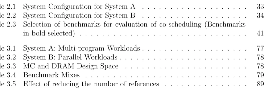
LIST OF TABLES

Table 2.1 System Configuration for System A . . . 33

Table 2.2 System Configuration for System B . . . 34

Table 2.3 Selection of benchmarks for evaluation of co-scheduling (Benchmarks in bold selected) . . . 41

Table 3.1 System A: Multi-program Workloads . . . 77

Table 3.2 System B: Parallel Workloads . . . 78

Table 3.3 MC and DRAM Design Space . . . 78

Table 3.4 Benchmark Mixes . . . 79

(13)

LIST OF FIGURES

Figure 1.1 Temporal and Spatial reuse at 64B block granularity shown with

var-ious strides. The machine configuration follows Table 2.1. . . 8

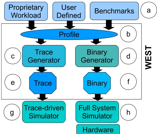
Figure 2.1 WEST Framework. . . 15

Figure 2.2 Global vs. Set Stack Distance in a 4-way cache. . . 20

Figure 2.3 Set Reuse profile with a depth of 8 in a 32KB L1 cache. . . 21

Figure 2.4 Fraction of writes across sets and stack positions. . . 22

Figure 2.5 Set Access Distribution (SAD) in a 32KB L1 cache with 128 sets . . 22

Figure 2.6 Co-scheduled behavior of 2 copies of hmmer in a 2M shared cache . . 25

Figure 2.7 Trace Generation Algorithm for a single memory reference (a), con-tents of various arrays before address generation (b) versus after ad-dress generation (c). . . 31

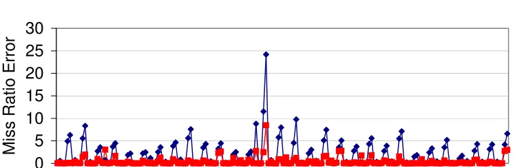
Figure 2.8 Comparison of miss ratio errors of GSD vs. WEST clones (Section 2.1.2) for various L1 cache configurations. . . 36

Figure 2.9 System A L1/L2 Cache Size DSE . . . 37

Figure 2.10 System A Set Change DSE . . . 38

Figure 2.11 System A Additional Cache Level . . . 39

Figure 2.12 System A Write Policy DSE . . . 40

Figure 2.13 System A Replacement Policy DSE . . . 40

Figure 2.14 Impact of varying L2 cache size on L2 miss ratio: benchmark 0 (left) & benchmark 1 (right). . . 42

Figure 2.15 Impact of varying L2 cache size on IPC: benchmark 0 (left) & bench-mark 1 (right). . . 43

Figure 2.16 Impact of varying L1 cache size on L2 miss ratio: benchmark 0 (left) & benchmark 1 (right). . . 44

Figure 2.17 Impact of varying L1 cache size on IPC: benchmark 0 (left) & bench-mark 1 (right). . . 45

Figure 2.18 System B (Out-of-order) Evaluation . . . 45

Figure 2.19 Trace Length Analysis . . . 46

Figure 3.1 DRAM Physical Hierarchy. Additional chips for reliability not shown for simplicity. . . 51

Figure 3.2 DRAM Logical View. . . 52

Figure 3.3 Address Mapping Schemes . . . 55

Figure 3.4 MEMST Framework. . . 57

Figure 3.5 DRAM addressing and analogy to cache addressing. . . 59

(14)

Figure 3.8 Example of inter-arrival gap showing an interleaved stream from two cores to a single row in a RIT. Inter-arrival gap shown between succes-sive transactions. Updates to timing distributions for core0 and core1 shown below. . . 64 Figure 3.9 Example of HPA for two streams of memory references. . . 64 Figure 3.10 Example of HIP for a stream of memory references from a single core

to a single row in the RIT. References interrupted by accesses from another core shown with arrows. . . 66 Figure 3.11 Symbiotic hits for parallel workloads . . . 67 Figure 3.12 Example of an interleaved stream of references from three cores. The

table shows TI[cx][cy]. . . 68

Figure 3.13 Example of two standalone streams from two cores interacting in a co-schedule. . . 70 Figure 3.14 State Diagram driving address generation. States generating addresses

are highlighted. . . 76 Figure 3.15 Multi-program workload evaluation: DRAM Organization DSE . . . 81 Figure 3.16 Multi-program workload evaluation: DRAM Address Mapping DSE . 81 Figure 3.17 Multi-program workload evaluation: DRAM Frequency DSE . . . 82 Figure 3.18 Multi-program workload evaluation: MC Transaction Scheduling

Pol-icy DSE . . . 83 Figure 3.19 Multi-program workload evaluation: MC Page Policy DSE . . . 84 Figure 3.20 Multi-program workload evaluation: DRAM Generation DSE . . . . 85 Figure 3.21 Multi-program workload evaluation: Bus Bandwidth and Chipset

(15)

Chapter 1 Introduction

(16)

space that includes choices in DRAM organization, address mapping policy, scheduling policy, etc. Hence, the design focus has been rapidly shifting from the core to the memory hierarchy.

To effectively evaluate the vast memory hierarchy design space, designers need to carefully select workloads. The choice of workloads is instrumental in driving key design decisions that influence performance, cost, power and schedule. Ideally, evaluation tech-niques should use workloads that are representative of end user workloads. Using an end user workload bolsters the confidence of both the designer and the end user because it helps the designer make workload-centric trade-offs and harden the design. However, end users are generally unwilling to share their workloads with designers. Access to source code is highly restricted due to the proprietary nature of applications. One example is a company with a proprietary trading algorithm that may be unwilling to share their code with designers. Another example is a highly classified weapons simulation code in a national lab which cannot be shared with most employees in the lab, let alone designers. A possible alternative to source code access is collecting a trace. Again, this is not a viable option because traces are generally very large in size and it is not possible for the end user to determine whether there is any confidential data captured in the trace. So, most end users are apprehensive about sharing code or traces due to the proprietary or confidential nature of code and data [21, 30]. This is called the proprietary workload problem. Thus, on one hand designers need in-depth insights into end user workloads, and on the other hand, end users cannot reveal any significant information about their code to designers.

(17)

SPECjbb2005 [7], TPCC [6], etc. have evolved over time in an effort to provide a com-mon framework to measure and compare performance. It is very comcom-mon for designers to use such benchmarks during the early design phase in a simulation environment. How-ever, benchmarks may not be either representative of proprietary workloads or may not exist at all [32, 30]. End users attach far more credibility to data collected using their workload as opposed to standard benchmarks [30]. So, industry-standard benchmarks do not address the issue of proprietary workloads. Another alternative to detailed simula-tions is statistical simulation [17, 18, 16, 26, 27, 38, 39]. Statistical simulation generates a short synthetic trace from a statistical profile of workload attributes such as branch misprediction rate, cache miss ratio, etc. The synthetic trace can be simulated using a statistical simulator to provide a performance estimate. The main benefit of this ap-proach is reduced simulation time. However, there are two important drawbacks of this technique. Firstly, the synthetic traces can only be used in statistical simulators not execution-driven simulators or real hardware. Secondly, their purpose is to cull very early designs and not to solve the proprietary workload problem. Another alternative is to build analytical models [33, 28, 19] to estimate performance. While analytical models can produce results quickly, it requires considerable effort to represent complex microar-chitectures with mathematical models. When the underlying architecture is changed, the analytical model has to be redesigned. So, similar to statistical simulation, they are gen-erally used in very early design. So, the existing techniques do not solve the proprietary workload problem and can not be used for detailed design work.

(18)

There are generally two approaches to cloning a workload: white boxorblack box. In a white box approach, subject experts gather as much information as they can from the end user, such as code behavior, algorithm, data characteristics, etc. and use the information to create a clone that hopefully produces behavior similar to the end user workload. The advantage of the white box approach is that it can ultimately yield an accurate clone, due to the accumulated experience of the subject experts, and feedback from the end users. The drawbacks of the white box approach are that it is highly manual, requires years of accumulated expertise and experience, and is riddled with potential pitfalls. For example, even with the knowledge of a particular graph algorithm, subject experts may still be unable to reproduce the cache behavior of the workload unless they use the correct data structure and layout in memory.

(19)

it or by using hardware analyzers/profilers. Whatever the profiling method may be, the only information exchanged between the end user and the design team is the workload profile. This solves the proprietary workload problem. The second challenging aspect of cloning is generation of the clone in the design environment using the profile provided by the end user. The clone must not only be able to accurately mimic the behavior of the profiled workload as the underlying architecture is changed, but should also be micro-architecture independent and portable. Micro-micro-architecture independence is achieved by selecting profiling statistics that are agnostic to the underlying hardware. For example, if statistics are selected that are dependent on the cache replacement policy, then the proprietary application has to be profiled again when the replacement policy is changed. This implies that statistics should model application behavior and not micro-architectural behavior. Portability of clones is achieved by using high-level languages like C, C++ or assembly-level directives.

The focus of this dissertation is black box workload cloning for exploring the memory hierarchy design space. We will first analyze statistics that are necessary to sufficiently capture application behavior. These statistics are collected when profiling workloads that may be proprietary in nature. We will also look at clone generation techniques, where we will show how a workload clone (trace/binary) can be generated using the collected profile. Finally, we will validate our profiling and clone generation techniques through extensive design space exploration of the underlying architecture.

(20)

goal of the dissertation is to build a cloning framework that enables cache designers to study and explore the cache design space using clones that are representative of end user workloads.

MC/DRAM is another important component in processor design. MC and DRAM-based memory are generally shared among multiple cores in a CMP. The bandwidth to main memory does not grow at the same pace as the number of cores due to pin limitations, power constraints or packaging costs [41]. So, as the number of cores increase, the contention for memory bandwidth also increases making it one of the key bottlenecks in the system. So, designers need a framework that allows them to effectively evaluate the numerous MC/DRAM design choices like memory organization, scheduling policy, page policy, DRAM frequency, etc. The second goal of the dissertation is to provide a cloning framework for modeling MC/DRAM behavior for proprietary workloads.

1.1 WEST: Cloning Data Cache Behavior using

Stochastic Traces

(21)

of statistics and then using these statistics, a clone is generated using an automated method. The clone can be used by the designer in place of the proprietary workload for studying cache designs.

Bell et al. [10] and Joshi et al. [30] are credited with pioneering work in the area of black box cloning forinstruction level parallelism behavior. They create clones by gener-ating instructions that replicate the original workload’s statistics in terms of instruction mixes, data flow graphs, and data dependence distance. Their contribution inspires this work into looking at whether we can clone data cache behavior accurately. While their work accurately captures instruction behavior, the data cache accesses are abstracted as a single dominant stride [30]. We found, however, that a single dominant stride is insufficient for representing a workload’s data cache behavior. Figure 1.1 shows the tem-poral and spatial reuse of CPU2006 [7] and BioBench benchmarks [8]. To characterize the memory references, we detected stride patterns at a cache block granularity for every memory reference and classified them based on the stride amount (stride amount of zero is classified as temporal reuse). The figure shows that for about 2/3 of the benchmarks, at least 90% of the accesses are temporal in nature. It also shows that for the remaining benchmarks, there are at least 3 dominant strides (>1% of total access) that account for the memory accesses. One of the benchmarks, tiger, has over 80% of memory accesses that are random in nature. Hence, capturing one dominant stride is insufficient to fully capture arbitrary access patterns for many workloads.

(22)

0 20 40 60 80 100 h 2 6 4 re f p e rl b e n c h c lu s ta lw c a c tu s to n to b w a v e s p h y

lip _gcc

s o p le x g a m e s s d e a l h m m s e a rc h m m e r le s lie c a lc u lix g ro m a c s s p h in x p o v ra y s je n g o m n e tp p x a la n fa s td n a lib q u a n tu m g e m s b z ip z e u s m p m u m m e r m

ilc _go

n a m d a s ta r lb m m c f ti g e r A c c e s s %

<-2 -2 -1 Temporal 1 2 3 4-7 8-15 16-31 32 >32

Figure 1.1: Temporal and Spatial reuse at 64B block granularity shown with various strides. The machine configuration follows Table 2.1.

was long believed to sufficiently capture any memory access pattern, and was used by various analytical models for predicting and explaining various cache performance phe-nomena, e.g. studies in [13, 14, 28, 34]. We show, however, that stack distance profile is necessary, but not sufficient. We found that in addition to stack distance profile, temporal locality across sets, access distribution across sets, and read/write distribution, need to be profiled at a fine granularity in order to capture data cache behavior. The combination of all these profiled statistics capture arbitrary memory access patterns very well. This is demonstrated in the following way: statistics profiled from one cache configuration enables the generation of a clone that produces nearly identical data cache statistics on multitudes of other single core cache configurations, such as different cache sizes, cache associativities, cache sets, cache write policies, replacement policies; and also a shared cache configuration in a CMP architecture.

(23)

identicalif they produce the same statistics under the machine configuration from which the statistics are profiled.

We evaluated WEST using the CPU2006 and BioBench benchmark suites over a wide cache design space for single core and dual core CMPs. In comparison to the profiled workloads, the clones, on average, had an error of 0.4% for miss ratio for 1394 single core cache configurations and 3.1% for miss ratio for over 600 co-scheduled configurations.

Other benefits of WEST include clone portability and short simulation time. Clones are highly portable because they are written using standard C-code and assembly lan-guage directives. WEST clones speed up execution by shrinking the number of instruc-tions in the original workload which range from millions to billions by orders of magnitude and still produce identical statistics.

To summarize, the key contributions of this work are:

1. An analysis of what key statistics are necessary and sufficient to represent data cache behavior.

2. A framework to generate statistically-identical clones to reproduce data cache be-havior.

3. An evaluation that demonstrates that clones generated using one cache configura-tion, can produce closely matching miss ratios and IPCs of the original benchmarks, on a wide range of other cache configurations, including a variety of sizes, associa-tivities, number of sets, write policies, replacement policies and different levels of caches.

(24)

the original benchmarks.

1.2 MEMST: Cloning Memory Behavior using

Stochastic Traces

The memory subsystem has been a key bottleneck in Chip Multi Processors (CMP) in terms of performance and power. With multiple workloads competing for memory capacity and bandwidth, Memory Controller (MC) and DRAM design is becoming very challenging. A good design should optimize for various end user workloads while meeting cost, power and schedule constraints. The importance of using end user workloads for characterizing and exploring design space instead of using industry-standard benchmarks is well-known [30, 20].

MC/DRAM designers need an in-depth understanding of end user workloads. His-torically, this has required either access to the source code or a trace. Getting access to source code or traces from the end user is rarely possible due to the proprietary nature of the source code or the confidential nature of data [9, 21, 30].

To solve this problem, designers use a reduced representation of the proprietary code. This miniaturized version is referred to as aclone. There are two approaches to cloning a workload: white boxorblack box[9]. The black box technique provides a convenient way to abstract the workload to a set of key statistics instead of needing detailed understanding of underlying code structure or algorithm. So, such cloning techniques are generally preferred for solving the proprietary workload problem.

(25)

models Instruction Level Parallelism (ILP) behavior. Balakrishnan and Solihin proposed a WEST framework to clone data cache behavior. Ganesan et al. [21, 24] extended the framework proposed by Bell et al. to capture Memory Level Parallelism (MLP) behavior and clone multi-threaded workloads. Prior cloning techniques have a limitation that they were not designed and cannot be used to extensively study and explore MC/DRAM design space. Cloning techniques in [10, 21, 24, 30] model the spatial locality of memory accesses by abstracting them as a single dominant stride per static load/store, but do not model temporal locality of memory behavior [9]. While WEST captures temporal locality in caches, WEST abstracts cache miss streams as random references, hence it does not capture temporal and spatial locality beyond the last level cache.

(26)

clones that can accurately mimic the original workload across a wide design space that includes varying organization, DRAM page sizes, ranks, channels, DDRx frequencies, MC page policy, MC scheduling policy, DRAM die revisions, DDRx generations and refresh policies. The analysis of statistics needed to replicate MC/DRAM behavior is the first contribution of this work.

A second contribution of this work is a unique clone generation technique. Modeling co-scheduling behavior in MC/DRAM requires generating parallelism at the thread-level and bank-level and ensuring appropriate serialization of requests to the same bank. This requires ensuring fine-grained coordination between the clones running on different cores to model co-scheduled behavior accurately. To achieve this, we propose to generate memory references using a parallel program and synchronize the threads using baton locks so that the timing of the arrivals and how accesses from different threads are interleaved are faithfully replicated.

One by-product of cloning is that MEMST can shrink the number of accesses of the original workload to a small fraction and still maintain a high degree of accuracy. This leads to much shorter simulation times, making design space exploration cheaper for MC/DRAM designers.

We evaluated MEMST using the CPU2006, BioBench, Stream and PARSEC bench-mark suites over a wide design space for single-core, dual-core, quad-core and octa-core CMPs. The clones were able to accurately represent the benchmarks for over 7900 data points with an average error of 1.8% and 1.6% for transaction latency and DRAM power respectively.

To summarize, the key contributions of this work are:

(27)

buffer miss ratio, memory bandwidth, transaction latency and DRAM power for proprietary workloads.

2. A novel cloning methodology to generate clones for exploring a wide MC and DRAM design space in simulators and hardware.

3. A comprehensive evaluation to validate the cloning technique in single-core, dual-core, quad-core and octa-core CMPs. The design space includes varying DRAM organization, address mapping, DDRx frequencies, MC page policy, MC scheduling policy, DRAM die revisions, DDRx

1.3 Organization of the Dissertation

(28)

Chapter 2 WEST: Workload Emulation using

Stochastic Traces

This chapter is organized as follows: Section 2.1 describes the profiling technique and clone generation methodology. Section 2.2 describes our evaluation methodology. Sec-tion 2.3 provides the results from our evaluaSec-tion and analyzes the findings. SecSec-tion 2.4 describes related work. Section 2.5 concludes this work.

2.1 WEST Framework

(29)

clone, a binary clone, or simply as aclone when it applies to both types.

Components of the WEST framework are shown in Figure 2.1. The profile must contain necessary and sufficient statistics needed for accurate clone generation. Custom user-defined profiles are also possible for generating clones for validation and debugging. The profile is fed to the trace generator (c) and the binary generator (d). The trace generator outputs a stream of memory references (e) that can be used in trace-driven simulators (g), while the binary generator creates an intermediate C program using the profile. The C program is then compiled to generate a binary (f), that can be used in full system simulators or real hardware (h).

_!

! "

"

!

(30)

2.1.1 Scope and Limitations

WEST aims to model data cache behavior for sequential programs running alone or co-scheduled on a CMP. Currently, WEST does not capture TLB behavior, coherence misses in parallel programs, instruction cache behavior, and cache pollution from instructions. Our primary goal is to match the miss ratio and IPC of the profiled workload when the underlying cache configuration is changed. We assume a simple processor model for IPC, using IPC as a mechanism to control rate of issue of accesses to the memory hierarchy. Producing IPC for a more complex, OoO processor model, requires not only reproducing data cache behavior, but also instruction level behavior, which is beyond the scope of this work. The data cache behavior cloned by WEST depends on the time period for which statistics are profiled. WEST can clone whole-program behavior as well as phase-specific behavior, if profiles are collected for each phase. WEST does not collect statistics for data cache behavior within a cache block, hence different profiling runs and clones are needed for different cache block sizes. Finally, we ignore the contribution of compulsory cache misses.

2.1.2 Analysis of Necessary and Sufficient Statistics

As discussed earlier, the black box approach to workload cloning does not require sub-ject expert knowledge and can be automated. However, one of the key challenges is to ensure that the profiled statistics that are used for generating the clone necessarily and sufficientlyrepresent the workload’s behavior. This section discusses our analysis of what statistics fully capture a workload’s data cache behavior.

(31)

data cache behavior of the application to be cloned. However, this fact still does not provide us an insight into how spatial reuse and temporal reuse can be measured, and what statistics are sufficient to represent them. Let us examine the two questions in more detail.

Spatial reuse represents the likelihood of accessing a consecutive datum in the near future. Prior studies in benchmark cloning attempt to discover a stride amount s such that when address x is accessed, x+s is the likeliest address to be accessed next by the program [30]. While such an approach has merit, Figure 1.1 shows that it is rare for arbitrary programs to exhibit memory access patterns with a dominant stride amount, especially at a cache block granularity. We will further argue that spatial reuse is sub-sumable by temporal reuse, consequently making it unnecessary to capture spatial reuse. There are several reasons for this.

First, intuitively, within a cache block, spatial accesses to adjacent words in the block will appear as multiple accesses to the same block. Thus, spatial reuse at a fine granularity manifests as temporal reuse at a coarser granularity. Secondly, any spatial block that is accessed, is also a block that has been accessed before, unless when the block is first accessed. This means that aside from the initial accesses, any access to a word or block is a temporal reuse of the word or block. Hence, excluding the initial accesses, spatial reuse is subsumedby temporal reuse. However, theconverse is not true. Some (or much) temporal reuse is not spatial reuse. Hence, capturing spatial reuse only such as the stride amount is clearly incomplete. Excluding the initial accesses is fine in most situations as they only cause compulsory cache misses, which are overwhelmed by orders of magnitude by other (capacity and conflict) cache misses.

(32)

distance measures the distribution of the number of distinct data elements accessed be-tween two consecutive references to the same element. Mattson et al. originally proposed stack distance profile as a way to measure misses for various storage structure sizes in one pass [36], for a fully-associative structure employing LRU replacement policy. Hill showed that stack distance profiling is also applicable to a set-associative cache, if the profile is collected for each set in the cache [29]. Many subsequent studies use stack distance profiles to predict various cache performance phenomena. For example, stack distance profile was used to predict the cache miss impact of cache sharing in CMP [13], predict the impact of prefetching on context switch misses [34], predict the performance of various cache replacement policies [28], predict throughput [14], and many others. The prevalence of the use of stack distance profile as thekeystatistic for predicting cache per-formance behavior indicates that conventional wisdom assumes that temporal reuse can be fully captured by the stack distance profile. In this work, we argue that, contrary to conventional wisdom, additional statistics are needed for fully capturing temporal reuse pattern of an application.

Let us start by reviewing what a stack distance profile captures. In a stack distance profile, the LRU stack position for each block is kept current at all time. For a cache with S sets, letCij denote the number of times data block located in the ith set and jth

stack position is accessed, where i = 1,2, . . . , S and j = 1,2, . . . ,∞. For simplicity of discussion, we assume that the stack distance profile keeps track of an unlimited number of ways.

(33)

Stack Distance(GSD) profile. We argue that despite its prevalence, conventional GSD profile provides insufficient information about the temporal reuse behavior. We use a subtly different stack distance profile, Set Stack Distance (SSD), that keeps one set of private values for each cache set, in order to capture temporal reuse behavior for each individual set. More formally, SSD(i, j) and GSD(j) can be expressed as:

SSD(i, j) = _P_∞Cij

j=1Cij

GSD(j) =

PS

i=1Cij

PS

i=1

P∞

j=1Cij

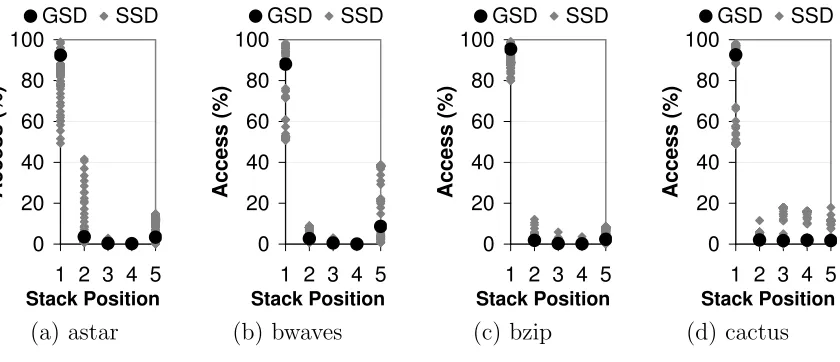
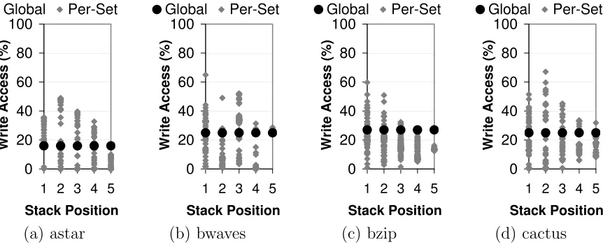
The reason to use SSD in lieu of GSD is due to the large variation of temporal reuse across sets. We illustrate this variation in Figure 2.2, which shows that the deviation in fractions of accesses that fall into a particular stack position can be very substantial: all 4 benchmarks show substantial deviation in the MRU position (> 18%) and in the miss position (> 8%). In the intermediate positions, cactus shows large deviations in all positions, astar shows only in the MRU-1 position while bwaves shows no major deviation. While only four benchmarks are shown, large deviations are common in other benchmarks. Therefore, GSD is insufficient for capturing the data cache behavior of an application, and SSD should be used instead.

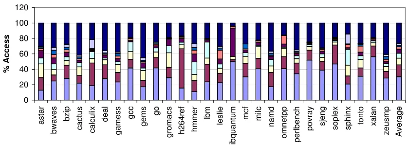
However, even SSD is necessary but insufficient to capture an application’s temporal behavior. This is because of our observation that there is a very strong locality across cache sets, where recently visited sets are more likely to be revisited. Figure 2.3 shows distribution of accesses to eight most-recently visited sets. The figure shows that indeed, temporal reuse is present across cache sets with an average of 30% of accesses to the most recently visited set. We will refer to this as Set Reuse(SR) Profile.

(34)

0 20 40 60 80 100

1 2 3 4 5

Stack Position A c c e s s ( % ) GSD SSD 0 20 40 60 80 100

1 2 3 4 5

Stack Position A c c e s s ( % ) GSD SSD

(a) astar (b) bwaves (c) bzip (d) cactus

Figure 2.2: Global vs. Set Stack Distance in a 4-way cache.

matches any of the H sets. Let SR(i) denote the number of times (in percent) that an access is to the same set as in the ith position in the window of H most recently visited sets, for i = 1,2, . . . , H. Let SR(H + 1) denote the number of times (in percent) that an access is to a set that is different than the most recent H sets. In profiling, we use

H = 8, because the reuse across sets falls sharply beyond this value.

(35)

0 20 40 60 80 100 120 a s ta r b w a v e s b z ip c a c tu s c a lc u lix d e a l g a m e s s g c c g e m s g o g ro m a c s h 2 6 4 re f h m m e r lb m le s lie lib q u a n tu m m c f m ilc n a m d o m n e tp p p e rl b e n c h p o v ra y s je n g s o p le x s p h in x to n to x a la n z e u s m p A v e ra g e % A c c e s s

MRU MRU-1 MRU-2 MRU-3 MRU-4 MRU-5 MRU-6 MRU-7 Other

Figure 2.3: Set Reuse profile with a depth of 8 in a 32KB L1 cache.

For these reasons, cloning data cache behavior requires reads and writes to be distin-guished. The remaining question is what statistics should be collected. There are three possibilities: fraction of accesses that are writes for the entire cache (global), fraction of accesses that are writes for each stack position for the entire cache (per-distance), and fraction of accesses that are writes for each set and each stack position (per-set). A global write fraction is sufficient if the write fraction is independent of stack position and does not vary across sets. A per-distance write fraction is sufficient if there is no variation across sets. We choose per-set write fraction because as shown in Figure 2.4, there is a significant variation in fraction of writes across stack positions and across sets (shown by the scatters), which cannot be captured by global or per-distance write statistics. We refer to the per-set profile as Write Fraction(WF).

Besides SSD, SR, and WF probability distributions, we also need to collect the dis-tribution of accesses to different sets, which we will refer to as Set Access Distribu-tion (SAD). SAD can be easily computed from SSD profile counters. More specifically:

SAD(i) =

P∞

j=1Cij

PS

i=1 P∞

(36)

0 20 40 60 80 100

1 2 3 4 5

Stack Position W ri te A c c e s s ( % ) Global Per-Set 0 20 40 60 80 100

1 2 3 4 5

Stack Position W ri te A c c e s s ( % ) Global Per-Set

(a) astar (b) bwaves (c) bzip (d) cactus

Figure 2.4: Fraction of writes across sets and stack positions.

As illustrated in Figure 2.5, certain sets are accessed far more frequently than others, with some sets receiving as much as 30% of the accesses. We observe similar behavior across all benchmarks, but only ten representative benchmarks are shown.

0

10

20

30

40 Benchmark

A

c

e

s

P

e

r

S

e

t

(%

)

Uniform Distribution

Actual Distribution

Figure 2.5: Set Access Distribution (SAD) in a 32KB L1 cache with 128 sets

(37)

will still reproduce data cache behavior when we add or subtract levels of caches, or when we change the configuration of the upper level caches which filter out accesses to the lower level caches (more in Section 2.3). So, the clone is generated to capture temporal reuse at all profiled cache levels. We will show that although we profile using an L1 and L2 cache, we can accurately predict miss ratios even when we change cache sizes to vary the amount of filtering from the higher level caches, change the number of sets at lower cache levels and add additional cache levels. An important question is whether SSD, SR, WF, and SAD should be collected for the different caches separately. This question determines whether the profiling should be performed at the L1 cache only, L1 and L2 caches, L1/L2/L3 caches, etc. The reason why this question is important is not because of profiling complexity since all the profiling statistics can be collected from a single execution/simulation run. The reason why this question is important is because it determines whether a clone that is generated while assuming a certain cache hierarchy will still reproduce data cache behavior when we add or subtract levels of caches, or when we change the configuration of the upper level caches which filter out accesses to the lower level caches.

(38)

errors remain very small.

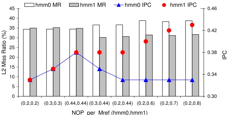
So far, we have made the case that SSD, SR, WF, and SAD are required to fully capture the temporal reuse pattern of a workload. These statistics are sufficient for a sequential workload running on a single core system. However, for workloads co-scheduled on a CMP where cores share a cache, we need one more statistic. With a shared cache, multiple streams of references from multiple upper level caches compete for cache space. In such a situation, the rate of memory references from each stream to the shared cache needs to be modeled. Figure 2.6 illustrates this with a case where two copies of the same clone are co-scheduled, with the rate of memory accesses varied by changing the underlying IPC of the cores. When the IPCs of the two benchmarks are equal, as expected, the clones achieve an equal miss ratio (shown in the first three columns). However, as the IPCs of the two copies diverge, the miss ratios also diverge. Therefore, it is important to capture the rates at which memory references are generated. The rate depends on the share of memory references in the original instruction stream, the relative speed of the processor cores, and instruction level parallelism. WEST clones do not produce instruction streams other than memory references. Hence, to control the rate, the distance between successive memory references must be controlled at the processor level. To achieve that, when the original benchmark is profiled, we capture the ratio of the total number of instructions to the total number of memory references. When the WEST clone is generated, the ratio determines how many NOPs should be inserted between consecutive memory references. We refer to this metric asNOP per Mref.

(39)

0 5 10 15 20 25 30 35 40 45

(0.2,0.2) (0.3,0.3) (0.44,0.44) (0.3,0.44) (0.2,0.44) (0.2,0.6) (0.2,0.7) (0.2,0.8)

NOP_per_Mref (hmm0,hmm1)

L

2

M

is

s

R

a

ti

o

(

%

)

0.30 0.34 0.38 0.42 0.46

IP

C

hmm0 MR hmm1 MR hmm0 IPC hmm1 IPC

Figure 2.6: Co-scheduled behavior of 2 copies of hmmer in a 2M shared cache

2.1.3 Generation Phase

In the previous section, we reduced the application’s data cache behavior to a set of statistics. The goal of this section is to explore how a clone, that reproduces the profiled statistics, can be generated. We distinguish between three approaches based on how closely clones approximate the profiled statistics: best effort,weak statistical convergence, and strict statistical convergence.

(40)

as the number of samples are increased. In contrast, in a strict statistical convergence, the clone produces statistics that exactly match the workload’s statistics. To illustrate the difference, consider a statistic of a workload that has a mean of 5. To achieve a weak convergence, a clone may be programmed to generate each sample independently from a statistical distribution with a mean of 5. The mean of individually generated samples may or may not be equal to 5, but over a large sample size will probabilistically converge to 5. In contrast, to achieve a strict convergence, the first sample is generated from the workload’s statistical distribution, but the distribution is adjusted before the second sample is generated, and this is repeated until the statistics match exactly. For example, if the sample size is two, and the first sample has a value of 0, then the second sample must have a value of 10, in order to force the mean of the two samples to be exactly 5.

The key benefits of strict convergence are that (1) statistical identity between the workload and its clone is guaranteed, and (2) it does not require a large sample size to achieve convergence. Hence, sample size can be scaled up or down while still guaranteeing statistical identity (subject to some constraints discussed in Section 2.3.4). Therefore, WEST adopts the strict statistical convergence approach and relies on a stochastic pro-cess that generates an acpro-cess stream from various statistical distributions.

(41)

Lxsubscript, wherexis the cache level. For example,SSDO,L2(i, j) denotes the original

Set Stack Distance profile at the L2 cache for the ith _{set and}_jth _{stack distance position.}

Initially, the input to the trace generation algorithm is the total number of accesses to be generated to different levels of caches (AL1, AL2). The value of ALx can be taken

from the original program profile, i.e. the number of accesses that produce the data cache behavior in the profile, or selected by users. Providing a user-specified value for

ALx is a significant feature of WEST, in that it allows users to scale down a long running

program with a very high number of accesses to a much shorter trace or binary clone, while remaining statistically identical to the original program, subject to some constraints (Section 2.3.4).

Given a scaling factor (scale), the first step of the algorithm is to scale down the number of accesses to all cache levels uniformly, i.e. AL1 = AO,L1 ×scale and AL2 =

AO,L2×scale.

2.1.4 Trace Clone Generation

The algorithm to generate the stochastic address trace is described below. For bookkeep-ing cache state, the generator uses a simple 2-level cache simulator identical to the one used by the profiler.

(42)

original workload is reached. The following arrays are initialized (with rounding):

SSDC,Lx(i, j) =ALx×SSDO,Lx(i, j) ∀i∀j

SRC,Lx(i) =ALx×SRO,Lx(i) ∀i

W FC,Lx(i, j) =ALx×W FO,Lx(i, j) ∀i∀j

2. Warmup: In this phase, we warm up the cache hierarchy by accessing a SL2×WL2

blocks sequentially, whereWLx and SLx denote the number of ways and sets of the

cache at level Lx.

3. Compute Cumulative Distribution Functions (CDF): Based on the Count Arrays, compute the various CDFs. The CDF arrays will be modified after each access is generated, to ensure strict statistical convergence regardless of the value of scale.

SSDCDF,Lx(i, j) =

Pj

k=1SSDC,Lx(i, k)

P∞

k=1SSDC,Lx(i, k)

∀i∀j

W FLx(i, j) =

W FC,Lx(i, j)

SSDC,Lx(i, j)

∀i∀j

SRCDF,Lx(i) =

Pi

k=1SRC,Lx(k)

PH+1

k=1 SRC,Lx(k)

∀i

SADCDF,Lx(i) =

Pi

k=1

P∞

j=1SSDC,Lx(k, j)

PSLx

k=1

P∞

j=1SSDC,Lx(k, j)

∀i

4. L1 Set Selection: Generate a random numberr ∈[0,1]. Comparer againstSRCDF

to determine which of the recently visited sets should be visited again. More specif-ically, find α1 such that SRCDF,L1(α1) ≤ r < SRCDF,L1(α1 + 1). If α1 is found,

(43)

that were recently visited. Hence, a new random numberr∈[0,1] is generated, and compared againstSADCDF,L1(·) to determine the set that is randomly selected, i.e.

SADCDF,L1(α1)≤r < SADCDF,L1(α1+ 1).

5. L1 Stack Position Selection: Generate a random number r ∈[0,1] and compare it

to SSDCDF,L1(α1,·) to select a stack position β1 such that SSDCDF,L1(α1, β1) ≤

r < SSDCDF,L1(α1, β1+ 1). If no suchβ1 is found, then we need to generate a miss

in the L1 cache.

6. L1 R/W Selection: Generate a random numberr ∈[0,1]. Ifr ≤W FL1(α1, β1), the

operation should be a write operation. Otherwise, it should be a read operation.

7. L1 Address Generation: If step 5 determined a cache miss, then go to step 8. To generate a hit in the L1 cache, we select the block in set α1 with the LRU

stack position β1 and generate an access to the block address. Based on what we

determined in step 6, the operation is a read or a write. Go to step 12.

8. L2 Set Selection: The selection of a set in the L2 cache is partially determined by the set selected in the L1 cache becauseα1 can only map to a certain group of sets

in the L2 cache. Thus, the set in the L2 cache must be selected from among the sets in this group. To do that, similar to the L1 set selection, a random number

r∈[0,1] is selected and compared toSADCDF,L2 to probabilistically determine the

selected set (α2). The process is repeated until the selected set is also one that

the L1 cache set maps to (the repeats can be avoided with minor mathematical transformations).

9. L2 Stack Position Selection: Generate a random number r ∈[0,1] and compare it

(44)

r < SSDCDF,L2(α2, β2+ 1). If no suchβ2 is found, then we need to generate a miss

in the L2 cache.

10. L2 Address Generation: If step 9 determined an L2 cache miss, then go to step 11. To generate a hit in the L2 cache, we select the block in set α2 with stack position

β2 and generate a read access to the block.

11. Memory Access Generation: Randomly generate a block address that maps to the set β2 but not already present in the L2 cache. When the memory footprint is

equal or larger than twice the size of the L2 cache, such an address can always be generated.

12. Adjust the Count arrays to account for the access just issued. The adjustment is by decrementing SSDC,L1(α1, β1), SRC,L1(α1), and W FC,L1(α1, β1) for the L1 cache.

The same is applied to the L2 cache, in the case of an L1 cache miss. If less than

AL1 accesses have been generated, go to step 3.

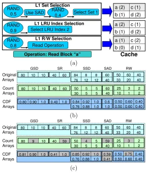
To illustrate the trace generation algorithm, Figure 2.7 shows a simple example of gener-ating a single memory reference for a cache with two sets and two ways. The addresses for blocks currently cached are shown in part (a) with the LRU stack position shown in parentheses. Assuming a user selects generation of 100 memory references, the initial values for the Count and CDF arrays, as well as Orig arrays, are shown in part (b). Sup-pose that the following random numbers will be generated: 0.5, 0.4, 0.9, and 0.8 from a random seed. To generate an address, the algorithm uses the first random number (0.5) and picks SRCDF index 2, which implies that a random set needs to be picked. Another

random number (0.4) is used to index into the SADCDF array and selects set 1. The

(45)

deter-mine an L1 cache hit. The final random number (0.8) is compared againstW FCDF(1,2)

to determine that the access is a read access. From part (a) in the figure, the algorithm determines that the access is a ”read to block a”. Part (c) shows how the various ar-rays are updated following the access. This procedure repeats until 100 addresses are generated. d (2) b (1) c (1) a (2) RAND

0.5 Use SAD RAND_0.4 Select Set 1

L1 Set Selection

RAND 0.9

L1 LRU Index Selection Select LRU Index 2

RAND

0.8 Read Operation

L1 R/W Selection

d (2) b (1) c (1) a (2) d (1) b (0) c (2) a (1)

Operation: Read Block “a” Cache

(a) GSD 20 60 40 33 40 50 12 8 12 76 8 84 10 10 80 40 60 60 40 SR 1 3 2 10 2 25 5 5 5 30 5 50 10 10 80 40 60 60 40 0.60 0.60 0.40 0.50 0.40 0.50 0.88 0.92 1.0 0.76 1.0 0.84 0.90 1.0 0.80 1.0 0.6 1.0 0.40

SSD SAD RW

Original Arrays Count Arrays CDF Arrays (b) GSD 20 60 40 33 40 50 12 8 12 76 8 84 10 10 80 40 60 60 40 SR 1 3 2 10 2 25 5 4 5 30 5 50 9 10 80 40 59 59 40 0.60 0.75 0.40 0.50 0.40 0.50 0.88 0.92 1.0 0.76 1.0 0.85 0.90 1.0 0.81 0.41 0.59 1.0 0.41

SSD SAD RW

Original Arrays Count Arrays CDF Arrays (c)

(46)

2.1.5 Binary Clone Generation

The binary clone generation process follows the same algorithm as trace generation. The output trace is modified by randomly distributing (N OP per M ref ×AL1) NOPs

between the AL1 accesses. In order to generate a C-program, the first step is to allocate

a large memory area that functions as the clone’s working set. Since our goal is to mimic the data cache behavior and not main memory behavior, we set the clone’s memory footprint at two times the size of the largest cache size that we will use in design space exploration. Keeping the memory at this size further improves simulation time. Then, all the NOPs and memory accesses in the trace are converted to asm directives in the C-program. The program is then compiled using a standard C compiler to generate the clone.

2.2 Evaluation Methodology

System Configuration. We use a full system simulation infrastructure based on Sim-ics [35] for our evaluation. We use “System A” with an in-order x86 processor for a wide design space exploration. The machine configuration used for profiling is shown in Table 2.1. The profiler is integrated into the Simics g-cache module and the statistics discussed in Section 2.1 are output to a file. All the benchmarks are profiledonceon Sys-tem A and the collected statistics are used to generate the benchmark clones offline. The binary clones are then compiled using gcc version 3.4.6. The benchmark and the binary clones are then used to explore numerous machine configurations shown in Table 2.1.

(47)

into the g-cache-ooo module. The profiling and clone generation method is identical to System B with profiles collected once for each benchmark and binary clones generated offline. The benchmark and the binary clones are then tested on different OOO machine configurations shown in Table 2.2.

The purpose of the wide design space exploration is to test whether the clones can still reproduce the data cache behavior of the original benchmark when it runs on machine configurations different from the one that was used for profiling. It is a validation of whether the statistics discussed in Section 2.1 sufficiently capture the behavior of the original workload for analyzing cache performance.

Table 2.1: System Configuration for System A

Profiling Test & Design Exploration

Cores 2 x86 cores, 2.0GHz, single issue

L1 I$/D$ Private 32KB, 4 way, LRU Private 8–32KB, 1–4 way, LRU WB w/ buffer (0 WB

penalty)

WT and WB w/ buffer (0 WB penalty)

2 cycles 2 cycles

L2$ 8MB, 32 way, WB, LRU 512KB–8MB, 2–32way,WB,

LRU/Rand

16 cycles 8–16 cycles

L3$ None 4–8MB, 16–32 way, WB, LRU

14-16 cycles

OS Fedora Core 10

Other 4GB memory with 100 cycle access, 64B block size (L1/L2/L3), MESI

(48)

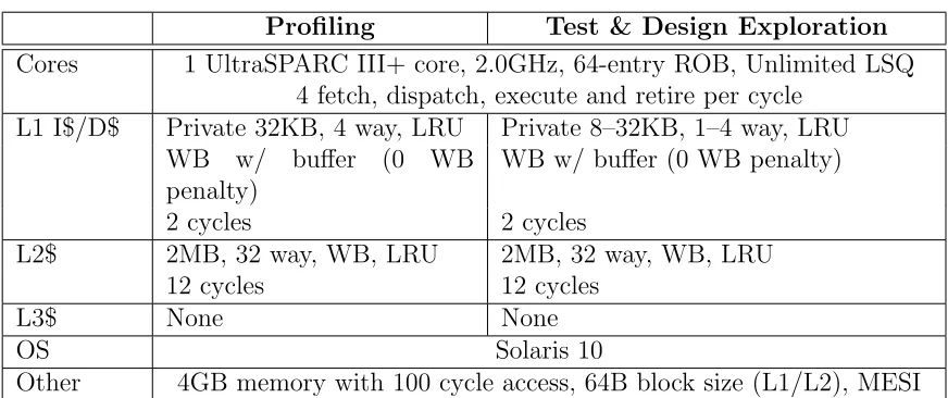
Table 2.2: System Configuration for System B

Profiling Test & Design Exploration Cores 1 UltraSPARC III+ core, 2.0GHz, 64-entry ROB, Unlimited LSQ

4 fetch, dispatch, execute and retire per cycle L1 I$/D$ Private 32KB, 4 way, LRU Private 8–32KB, 1–4 way, LRU

WB w/ buffer (0 WB penalty)

2 cycles 2 cycles

L2$ 2MB, 32 way, WB, LRU 2MB, 32 way, WB, LRU

12 cycles 12 cycles

L3$ None None

OS Solaris 10

Other 4GB memory with 100 cycle access, 64B block size (L1/L2), MESI

benchmarks were fast-forwarded for 5B instructions, warmed up for 250M instructions and after clearing statistics, run for 2B instructions on System A and for 250M instruc-tions on System B. The benchmark clones are run for one full iteration to avoid ITLB misses and instruction page faults. After that, statistics are cleared and they are run to completion. For co-scheduled workloads, the clones warm up together. Clones that complete warm-up earlier are halted until the last clone completes warm-up. The clones are then run to completion with each clone halted after it completes execution.

(49)

clones in the virtual address space is identical to the behavior exhibited in the physical address space after address translation.

Kernel transactions account for approximately 1%-2% of memory references across 1 billion memory references. Although this is amortized over such a large number of references, it can have an impact on the accuracy of WEST, especially with small traces. So, during WEST simulations, we allow the kernel transactions to access the cache but they are excluded from statistics. For the main benchmark simulations, we include the kernel transactions in the statistics to account for any system calls.

The memory footprint of the main benchmark is captured during the profiling phase but we chose to not utilize it for the evaluation. WEST only requires a memory footprint that is larger than the size of the largest cache (8MB in our evaluation) to allow generation of memory accesses. Since the profiled workloads had a footprint much larger than the last level cache size and allocation of large memory has significant simulation overhead, we chose to use a memory footprint of 16MB for our evaluation.

2.3 Results and Analysis

(50)

Figure 2.8 contrasts the result of clones generated using Global Stack Distance profile (GSD clone), the most commonly used statistic in literature for analyzing temporal reuse, versus clones generated using statistics that we proposed in Section 2.1.2. For this, we vary the L1 cache from 32K/4way to 16K/4way, 8K/4way, 16K/2way, 8K/2way and 8K/1way for both GSD clones and WEST clones. We observe that the GSD clones show significant errors in miss ratio (measured as the absolute difference in miss ratios) at many data points, reaching as high as 24%. WEST clones, on the other hand, show near-zero errors across almost all cases, and only shows a single point with a relatively elevated error. This result demonstrates that as we argued in Section 2.1.2, necessary and sufficient statistics must be used to generate an accurate clone. GSD is only necessary, but insufficient for that purpose.

0 5 10 15 20 25 30

Mi

s

R

a

ti

o

E

rr

o

r

GSD WEST

(51)

2.3.1 Results on Single Core (System A)

L1/L2 Cache Size

Figures 2.9 (a),(b),(c) show the L1 and L2 miss ratios, and IPC, obtained from the clones and the actual benchmarks, as the size of the L1 (8K/1way, 16K/2way, 32K/4way) and L2 caches (512K/2way, 1M/4way, 2M/8way, 4M/16way, 8M/32way) are changed. The figures show that the clones generate near identical results compared to those from the actual benchmarks across 510 runs. The average error in miss ratio (measured as the average of absolute differences in miss ratios) are 0.068% and 0.28% for the L1 and L2 caches, respectively. The average IPC error (measured as the average of absolute differences in IPCs) is only 0.002.

0 0.1 0.2 0.3 0.4 0.5

Benchmark WEST

0 0.2 0.4 0.6 0.8 1

Benchmark WEST

(a) L1 Miss Ratio (b) L2 Miss Ratio

0.1 0.3 0.5 0.7

Benchmark WEST

(c) IPC

(52)

Number of Sets

Figures 2.10 (a),(b) compare the L2 miss ratio and IPC of clones versus benchmarks when the number of sets in the L2 cache are varied, by fixing the cache associativity at 32 but varying the cache size from 2MB to 8MB. The average L2 miss ratio and IPC error are 0.59% and 0.0028 respectively. Only in two instances, the error is slightly elevated (9%). Changing the number of sets is challenging because when the number of sets are reduced or increased, the mapping of addresses to cache sets change, leading to changes in the SSD profile. However, as the figure shows, WEST can accurately mimic the benchmark behavior even when the number of sets in the L2 cache are changed, i.e. when the SSD in the original profile no longer matches those in the test runs.

0 0.2 0.4 0.6 0.8 1

Benchmark WEST

0.1 0.3 0.5 0.7

Benchmark WEST

(a) L2 Miss Ratio (b) IPC

Figure 2.10: System A Set Change DSE

Additional Cache Level

(53)

0 0.2 0.4 0.6 0.8 1

Benchmark WEST

0 0.2 0.4 0.6 0.8 1

M

is

s

R

a

ti

o

Benchmark WEST

(a) L2 Miss Ratio (b) L3 Miss Ratio

0.1 0.3 0.5 0.7

Benchmark WEST

(c) IPC

Figure 2.11: System A Additional Cache Level

we show the miss ratios only for those benchmarks where the L3 cache receives more 1% of the accesses. However, we show the IPC for all the runs in (c). When a clone produces very few accesses to the large L3 cache, miss ratios can show a large swing in values. Fundamentally, convergence cannot be ensured with too small a sample size (more discussion in Section 2.3.4). However, IPC is not affected by the swing in miss ratios because the number of accesses are very few. We observe errors of 0.25%, 0.83% and 0.0035 in L2 miss ratio, L3 miss ratio and IPC respectively.

Write Policy

(54)

0 0.2 0.4 0.6 0.8 1

Benchmark WEST

0 0.1 0.2 0.3 0.4 0.5 0.6 0.7

Benchmark WEST

Figure 2.12: System A Write Policy DSE

Replacement Policy

We switch the replacement policy used in the L2 cache from LRU to Random and vary the L2 cache size from 1-4MB. Figure 2.13 (a) shows an average error of 0.28% in L2 miss ratio. The average IPC error is only 0.002. There are some cases where the error is as high as 8%. For some of these pathological cases, the random replacement policy performs better than the LRU policy and the clone does not fully capture this outcome.

0 0.2 0.4 0.6 0.8 1

Benchmark WEST

0.1 0.2 0.3 0.4 0.5 0.6 0.7

IP

C

Benchmark WEST

Figure 2.13: System A Replacement Policy DSE

2.3.2 Results for Co-schedules on CMPs (System A)

(55)

co-scheduled, versus when the actual benchmarks run co-scheduled. We assume a 2-core CMP with each core having a private L1 cache and both cores sharing an L2 cache. To construct co-schedules, we categorize the 28 CPU2006 benchmarks based on their L1 miss ratio, L2 miss ratio, and IPC, when they run stand-alone (Table 2.3). We selected as many benchmarks necessary to get a good representation from each bin. Overall, we selected 15 benchmarks and mixed them in every possible combination for a total of 120 mixes. Due to space constraints, we will only show miss ratio charts in this section but we will discuss IPC results.

Table 2.3: Selection of benchmarks for evaluation of co-scheduling (Benchmarks in bold selected)

By L1 Miss Ratio By L2 Miss Ratio By IPC

Cord. Benchmark Cond. Benchmark Cond. Benchmark

<5%

bzip, calculix, gcc, go,

gromacs, h264, libqtm,

povray, sjeng, soplex,

tonto

<1%

astar, calculix, deal,

gamess, gromacs, h264,

hmmer, namd, perl,

povray, tonto

<0.3

bwaves, cactus, gems,

hmmer, lbm, leslie,

libqtm,mcf, milc, sphinx

5%-10%

astar, cactus, deal,

gamess, milc, namd,

omnetpp, perl, xalan,

zeus

1%-10%

bzip, cactus, gcc, gems,

go, soplex, sphinx,xalan

0.3-0.4

astar, bzip, gamess, gcc,

h264

>10% bwaves, gems, hmmer,

lbm, leslie,mcf, sphinx >10%

bwaves, lbm, leslie,

libqtm, mcf, milc,

om-netpp, sjeng,zeus

>0.4

calculix, deal, gromacs,

go, namd, omnetpp,

perl, povray, sjeng,

soplex, tonto,xalan,zeus

L2 Cache Size

(56)

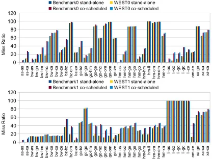
re-sults). The figures show a very close match between co-scheduled clones vs. co-scheduled benchmarks. The clones correctly reflect large increases in miss ratios whenever the benchmarks show such behavior, resulting in near-identical IPCs. The average error in L2 miss ratio for benchmark 0 and benchmark 1 across all 360 simulations was 3.4% and 3.1% respectively. The average error in IPC for the benchmarks is less than 0.01.

a s-as a s-xa bw -a s bw -g o bw -h m b w -m c bw -x a bw -x a bw -z e b z-bz bz -o m b z-ze g c-bz gc -g o g c-h m g o -g e g o -m c go -o m g o -o m go -z e h m -a s h m -b z h m -g e h m -g e h m -g o h m -h m hm -li hm -o m h m -o m h m -x a li-a s li-b z li-g o li-g o li-ze o m -z e xa -g e xa -x a xa -x a 0 20 40 60 80 100 120

Benchmark0 stand-alone WEST0 stand-alone

Benchmark0 co-scheduled WEST0 co-scheduled

M is s R a tio a s-as a s-xa bw -a s bw -g o bw -h m b w -m c bw -x a bw -x a bw -z e b z-bz bz -o m b z-ze g c-bz gc -g o g c-h m g o -g e g o -m c go -o m g o -o m go -z e h m -a s h m -b z h m -g e h m -g e h m -g o h m -h m hm -li hm -o m h m -o m h m -x a li-a s li-b z li-g o li-g o li-ze o m -z e xa -g e xa -x a xa -x a 0 20 40 60 80 100 120

M is s R a tio

(57)

0 0.1 0.2 0.3 0.4 0.5 a s -a s a s -x a b w -a s b w -g o b w -h m b w -m c b w -x a b w -x a b w -z e b z -b z b z -o m b z -z e g c -b z g c -g o g c -h m g o -g e g o -m c g o -o m g o -o m g o -z e h m -a s h m -b z h m -g e h m -g e h m -g o h m -h m h m -l i h m -o m h m -o m h m -x a li-a s li-b z li-g o li-g o li-z e o m -z e x a -g e x a -x a x a -x a

Benchmark0 coscheduled WEST0 coscheduled

0 0.1 0.2 0.3 0.4 0.5 a s -a s a s -x a b w -a s b w -g o b w -h m b w -m c b w -x a b w -x a b w -z e b z -b z b z -o m b z -z e g c -b z g c -g o g c -h m g o -g e g o -m c g o -o m g o -o m g o -z e h m -a s h m -b z h m -g e h m -g e h m -g o h m -h m h m -l i h m -o m h m -o m h m -x a li-a s li-b z li-g o li-g o li-z e o m -z e x a -g e x a -x a x a -x a

Figure 2.15: Impact of varying L2 cache size on IPC: benchmark 0 (left) & benchmark 1 (right).

L1 Cache Size

For the 120 co-schedules, we vary the L1 cache size between 8KB and 16KB while keeping the L2 cache size fixed at 2MB. Although the L1 cache is private to each core, varying the L1 cache size allows us to evaluate the co-schedule behavior when the filtering effect of the L1 cache is varied. Figure 2.16 shows the L2 miss ratio for the benchmarks running on core 0 and core 1. Out of a total of 240 simulations, only when at least one benchmark in a co-schedule suffers from an increase in L2 miss ratio change of over 5%, the result is shown (excluded cases show near-identical results). Again, the results show a very close match between co-scheduled clones vs. co-scheduled benchmarks. The average error in L2 miss ratio for benchmark 0 and benchmark 1 across all 240 simulations was 2.3% and 3.3% respectively. The average error in IPC for the benchmarks is less than 0.01.

2.3.3 Results on Single Core (System B)

(58)

a s-as as -g e a s-xa a s-ze bw -a s bw -a s bw -b z bw -b z bw -c a bw -g o b z-bz bz -g e bz -g e b z-o m b z-ze ca -l i ca -m c g c-a s g c-xa g o -m c go -x a h m -a s li-a s li-a s li-b z li-b z li-g o o m -z e o m -z e ze -x a 0 20 40 60 80 100 120

M is s R a tio a s-as as -g e a s-xa a s-ze bw -a s bw -a s bw -b z bw -b z bw -c a bw -g o b z-b z bz -g e bz -g e b z-om b z-ze ca -l i ca -m c gc -a s g c-xa g o -m c go -x a h m -a s li-a s li-a s li-b z li-b z li-g o o m -z e o m -z e ze -x a 0 20 40 60 80 100 120

M is s R a tio

Figure 2.16: Impact of varying L1 cache size on L2 miss ratio: benchmark 0 (left) & benchmark 1 (right).

fixed at 2M. As shown in Figure 2.18. we observe that the clones are accurate with an average error of 0.71% and 0.82% for L1 miss ratio and L2 miss ratio respectively.

2.3.4 Impact of Trace Length on Convergence

(59)

0 0.2 0.4 0.6 0.8 a s -a s a s -g e a s -x a a s -z e b w -a s b w -a s b w -b z b w -b z b w -c a b w -g o b z -b z b z -g e b z -g e b z -o m b z -z e c a -l i c a -m c g c -a s g c -x a g o -m c g o -x a h m -a s li-a s li-a s li-b z li-b z li-g o o m -z e o m -z e z e -x a

Figure 2.17: Impact of varying L1 cache size on IPC: benchmark 0 (left) & benchmark 1 (right). 0 0.1 0.2 0.3 0.4 0.5 Benchmark WEST 0 0.2 0.4 0.6 0.8 1 Benchmark WEST

(a) L1/L2 Cache Size: L1 Miss Ratio (b) L1/L2 Cache Size: L2 Miss Ratio Figure 2.18: System B (Out-of-order) Evaluation

that is too small may be insufficient to mimic behavior at the L1 cache (L1 sparseness), and, depending on the L1 miss ratio, at the L2 cache (L2 sparseness). The inaccuracy that arises due to sparseness is unrelated to the intrinsic ability of a clone to reproduce a workload’s data cache behavior.

(60)

500K and 2M memory accesses. The numbers above the columns denote the number of references for each Miss stack position averaged across all sets. As seen in Figure 2.19, the sparseness problem occurs as the number of references for the Miss stack position decreases below 10. In the case of the L1 cache, the Miss stack position sees only 1% and 5% of total references for profiles A and B respectively and the small miss ratios cause higher errors (L1 sparseness) as the trace size decreases. The L2 cache has far greater number of stack positions than the L1 cache (64×) and receives far fewer accesses due to the filtering effect of the L1 cache (L2 sparseness). This implies that more memory references are needed to achieve stochastic convergence at the L2 cache. In conclusion, it is important to maintain a trace size that is sufficiently large to achieve accuracy in all significant stack positions at all cache levels to achieve stochastic convergence.

0 0 1 7 31 0 0.01 0.02 2 0 0 0 5 0 0 1 0

0 ₃2 8

Trace Length(K) WEST Benchmark 0 0 1 4 17 0 0.5 1 2 00 0 5 00 1 0

0 ₃2 8

Trace Length(K) WEST Benchmark 0 2 9 46 186 0 0.02 0.04 0.06 2 0 0 0 50 0 1 0

0 ₃2 8

Trace Length(K)

WEST Benchmark

70 17 3 1 0 0 0.5 1 2 00 0 5 0 0 1 0 0

32 8

Trace Length(K)

WEST Benchmark

(a) Prof A: L1 Miss (b) Prof A: L2 Miss (c) Prof B: L1 Miss (d) Prof B: L2 Miss

Ratio Ratio Ratio Ratio

Figure 2.19: Trace Length Analysis

Workload Cloning: Emulating Memory Hierarchy Behavior using Stochastic Traces.

ABSTRACT

DEDICATION

BIOGRAPHY

ACKNOWLEDGEMENTS

TABLE OF CONTENTS

LIST OF TABLES

LIST OF FIGURES

Chapter 1

Introduction

1.1

WEST: Cloning Data Cache Behavior using

Stochastic Traces

1.2

MEMST: Cloning Memory Behavior using

Stochastic Traces

1.3

Organization of the Dissertation

Chapter 2

WEST: Workload Emulation using

Stochastic Traces

2.1

WEST Framework

2.1.1

Scope and Limitations

2.1.2

Analysis of Necessary and Sufficient Statistics

0

10

20

30

40

Benchmark

A

c

c

e

s

s

P

e

r

S

e

t

(%

)

Uniform Distribution

Actual Distribution

2.1.3

Generation Phase

2.1.4

Trace Clone Generation

2.1.5

Binary Clone Generation

2.2

Evaluation Methodology

2.3

Results and Analysis

2.3.1

Results on Single Core (System A)

2.3.2

Results for Co-schedules on CMPs (System A)

2.3.3

Results on Single Core (System B)

2.3.4

Impact of Trace Length on Convergence

2.4

Related Work