A GRAVITATIONAL SEARCH ALGORITHM-BASED OPTIMIZATION APPROACH APPLIED TO CAPACITOR PLACEMENT IN DISTRIBUTION SYSTEM

574 | P a g e

A GRAVITATIONAL SEARCH ALGORITHM-BASED

OPTIMIZATION APPROACH APPLIED TO

CAPACITOR PLACEMENT IN DISTRIBUTION

SYSTEM

Amanpreet Kaur

, Amarjeet Kaur

1

Student, Electrical Engineering, M.tech Power Engineering, (India)

2

Professor, Electrical Engineering, (India)

ABSTRACT

The power distributed into the network has losses, which is greater in distribution system compared to transmission system. Capacitors have been employed to provide reactive power compensation in distribution systems to resolve this problem. These are used to reduce power losses and to maintain the voltage profile within acceptable limits. The benefit of compensation depends greatly on how the capacitors are placed in the system, specifically on the location and size of the added or placed capacitors. So for this adopts two methods where the first method being the sensitivity analysis and the second method is the Gravitational Search Algorithm (GSA). Sensitivity analysis is a methodical technique, which is used to reduce the search space and to arrive at an accurate solution for recognizing the locality of capacitors. Capacitor values are allocated for the respective locations using GSA. The performance of the proposed method is scrutinized on distribution systems. It is applied to IEEE-33 and it is found that power losses in distribution system have been minimized. Due to which a significant amount of annual savings maximized. The techniques has been implemented in MATLAB R2014b environment.

Keywords: CBs-Circuit Breakers, DGs-Distribution Generators, GSA - Gravitational Search

Algorithm, PGSA – Plant Growth Search Algorithm, RDN-Radial Network

I.

INTRODUCTION

Electrical energy is produced in generators, transformed to an appropriate voltage level in transformers and then

dispatched via the buses on the transmission lines for final distribution to the loads. The circuit breakers allow

the tripping of faulty elements and also sectionalizing of the system. High voltage is being generated,

transformed, transmitted and distributed as three phase AC power. However AC power has several distinct

disadvantages. In AC circuits, the power factor is the ratio of the real power that is used to do work and the

apparent power that is supplied to the circuit. The power factor can get values in the range from 0 to 1. When all

the power is reactive power with no real power (usually inductive load) - the power factor is 0. Reactive power

is either generated or consumed in almost every component of the system, generation, transmission, and

distribution and eventually by the loads. In fact, reactive power is a liability on the source because the source

575 | P a g e

Most of the loads (e.g. induction motors, arc lamps, fluorescent lamps etc.) are inductive in nature and hence

have low lagging power factor. The low power factor is not desirable as it cause an inflation in current, resulting

in additional losses of active power in all the elements of power system from power station generator down to

the utilization devices. In order to ensure most favorable conditions for supply system from engineering and

economical standpoint, it is important to have power factor as close to unity as possible.It is economical to

supply this reactive power closer to the load in the distribution system. This can be achieved by installing

capacitor at appropriate location with suitable size. Capacitor Banks are commonly employed to provide

reactive power compensation in distribution network. The installation of capacitor banks involves determination

of size (kVAr ratings), location of capacitors. Selecting the best location for the capacitor will reduce the

requirement of the reactive power, which consequently maximizes the net savings and also used to maintain

voltage profile within permissible limits. To find out the potential locations for compensation, Loss Sensitivity

Factors (LSFs) are used. These factors are computed using sensitivity analysis. Using LSF, the candidate

number of buses are recognized. Gravitational Search Algorithm (GSA) employed in this paper is to choose the

optimized capacitor settings to be installed in the respective candidate buses which are obtained through LSF.

The proposed algorithm.

In 2015 Mohamed Shuaib adopted two method first was sensitivity analysis to find out the location of capacitor

and second one was GSA that determined the size of placed capacitor. Computational outcomes showed that the

proposed method is capable of generating optimal solutions.[1] K.R. Devabalaji et.al proposed a new long term

scheduling for optimal allocation of capacitor bank in radial distribution system with the objective of

minimizing power loss of the system subjected to equality and in equality constraints. In the proposed method

the new integrated approach of Loss Sensitivity Factor (LSF) and Voltage Stability Index (VSI) were

implemented to determine the optimal location for installation of capacitor banks. Bacterial Foraging

optimization algorithm (BFOA) was proposed to find the optimal size of the capacitor in 2015. [2] During 2013

Mohd Sabri et.al analyzed a Gravitational Search Algorithm (GSA) which is a recent algorithm that hasbeen

inspired by the Newtonian‟s law of gravity and motion. Sinceits introduction in 2009, GSA has undergone a lot

of changes to thealgorithm itself and has been applied in various applications. The authors were intended to dig

out the algorithm‟s current stateof publications, advances, its applications and discover its futurepossibilities.

This review is expected to provide an outlook on GSAespecially for those researchers who are keen to explore

thealgorithm‟s capabilities and performances. [3]

Shaw et al. in the year 2012 proposed a Gravitational search algorithm (GSA) that was based on the law of

gravity and interaction between masses. Authors proposed a novel algorithm to accelerate the performance of

the GSA. The analyzed opposition-based GSA (OGSA) of the work employed opposition-based learning for

population initialization and also for generation jumping. In the presented work, opposite numbers have been

utilized to improve the convergence rate of the GSA. The results obtained confirm the potential and

effectiveness of the proposed algorithm compared to some other algorithms surfaced in the recent state-of-the

art literatures. Both the near-optimality of the solution and the convergence speed of the proposed algorithm

were promising.[4] In the year 2012 Mohammad Khajehzadeh and Mahdiyeh Eslami developed a heuristic

global optimization algorithm called gravitational search algorithm (GSA). It is applied for the optimization of

576 | P a g e

the proposed method could provide solutions of high quality, accuracy and efficiency and outperforms other

methods for optimum design of retaining structure.[5] The success of Plant Growth Simulation Algorithm

(PGSA) with loss sensitivity factor to solve optimization problem was applied to capacitor placement by R.

Srinivasas Rao et.al in 2011, in which the objective function and the constraints separately handled and avoided

the trouble to determine the barrier factors. The proposed method has outperformed the other methods in terms

of the quality of solution. [6]

II.

PROBLEM

FORMULATION

The objective is to minimize the annual cost incurred due to kW losses and the annual cost due to capacitor

installations, subjected to certain operating constraints. The objective function does not include the operation

and maintenance costs of the capacitor placed in Radial network. The three phase system is considered as

balanced and loads are assumed as time invariant.

Mathematically, the objective function of the problem is described as:

minf = min (COST) (1)

Where COST is the objective function which includes the cost of power loss and the capacitor placement. The

voltage magnitude at each bus must be maintained within its limits and is expressed as:

Voltage constraints will be taken into justification by stipulating the Lower and Upper bound between Vmin =

0.95 p.u. and Vmax = 1.0 p.u.

Vmin≤│Vi│≥Vmax (2) The total kW losses of RDN having „N‟ buses and „N-1‟ branches is given by:

𝑃𝑇𝑜𝑡𝑎𝑙𝑙𝑜𝑠𝑠= 1≤ n≥N 1≤ m≥N𝑃𝑚𝑛 𝑙𝑜𝑠𝑠 (3)

The total energy loss cost (𝐸𝑐𝑜𝑠𝑡) has been calculated as:

𝐸𝑐𝑜𝑠𝑡 = 𝑃𝑇𝑜𝑡𝑎𝑙𝑜𝑠𝑠 ∗ 𝐾𝑝(4)

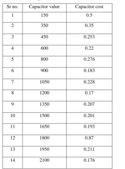
In general, the cost per KVAR varies with respect to their size. The available capacitor sizes and their cost (K)

were given in table 1. The total cost of the distribution system is given in Eq. (5).

𝐶 = 𝐸𝑐𝑜𝑠𝑡 + 𝐶𝑞𝑐𝑜𝑠𝑡(5)

Where,

𝐶𝑞𝑐𝑜𝑠𝑡 = 𝐾𝑓𝑐𝑐 ∗ 𝑄𝑖(6)

The percentage saving of the annual operating cost has been calculated using the Eq. (7) shown below,

%saving = (𝑖𝑛𝑖𝑡𝑎𝑙 𝑜𝑝𝑒𝑟𝑎𝑡𝑖𝑜𝑛 𝑐𝑜𝑠𝑡 −𝑓𝑖𝑛𝑎𝑙 𝑜𝑝𝑒𝑟𝑎𝑡𝑖𝑛𝑔 𝑐𝑜𝑠𝑡 )_{(𝑖𝑛𝑖𝑡𝑖𝑎𝑙 𝑜𝑝𝑒𝑟𝑎𝑡𝑖𝑛𝑔 𝑐𝑜𝑠𝑡 )} (7)

The mathematical statement of the problem can be conveyed by the following expression. [1]

𝑀𝑖𝑛𝑖𝑚𝑖𝑧𝑒 𝐹 𝑃𝑇𝑜𝑡𝑎𝑙𝑙𝑜𝑠𝑠 ∗ 𝐾𝑝 + [𝐾𝑓𝑐𝑐 ∗ 𝑄𝑖](8)

III. OBJECTIVES

The objectives of thesis are summarized as:

1) To identify the optimal location and size of capacitors to minimize the losses and cost of power loss in

577 | P a g e

2) Implementing Gravitational search Algorithm to find the optimal solution.

IV.

METHODOLOGY

The solution methodology has two steps:

1) In first step sensitivity analysis [6, 7]is considered in order to reduce the search space and to arrive at an

accurate solution for recognizing the locality.

2) In second step Gravitational Search Algorithm (GSA) is used to estimate the optimal size of capacitor.

Load flow

Load flow analysis is concerned with describing the operating state of an entire power system. Computational

procedure required to determine the steady-state operating characteristics of a power system network is termed

load flow. The aim of load flow calculations is to determine the steady state operating characteristics of power

generation/transmission system for a given set of bus bar loads. The main information obtained from the load

flow study is:

1) Magnitude and phase angles of load bus voltages

2) Reactive powers and voltage phase angles at generator buses

3) Real power and reactive power flow

4) Power at the reference bus

Here Newton-Raphson is used to calculate the losses of the network and power flows in the line. [8]

Sensitive analysis

The sensitivity analysis is a methodical technique to find out those locations with maximum influence on the

system active power losses with respect to the node reactive power. Sensitivity analysis is carried out also to

find the Loss Sensitivity Factor. The Loss Sensitivity Factoris so important that the candidate number of buses

are recognized.

Loss Sensitivity Factor (LSF)

To identify the location for capacitor placement in distribution system Loss Sensitivity Factors is used. LSF is

able to predict which bus will have the biggest loss reduction when a capacitor is placed. Therefore, these

sensitive buses can serve as candidate buses for the placement of capacitor. The estimation of these candidate

buses basically helps in reducing of the search space for the optimization problem. As only few buses can be

candidate buses for compensation, the installation cost on capacitor scan also be curtailed.

Consider a distribution line with an impedance (r + jx) and a load of (Peff& Qeff) connected between (i) and (j)

buses. (Peff& Qeff) are the active and Reactive power beyond the receiving end bus.

KW loss in the line is given by (I2ij * Rij), which can also be expressed as, [1]

𝑃𝑙𝑖𝑛𝑒𝑙𝑜𝑠𝑠 =

(𝑃_{𝑒𝑓𝑓𝑗}2 +𝑄_{𝑒𝑓𝑓𝑗}2 )∗𝑟_𝑖𝑗

𝑉_𝑗 2 (9)

Similarly the Reactive power loss in the line is given by:

𝑄𝑙𝑖𝑛𝑒𝑙𝑜𝑠𝑠 =

(𝑃_{𝑒𝑓𝑓𝑗}2 +𝑄_{𝑒𝑓𝑓𝑗}2 )∗𝑟_𝑖𝑗

𝑉_𝑗 2 (10)

Where

578 | P a g e

Qeff= Total effective reactive power supplied beyond the bus „j‟.

Now, the Loss Sensitivity Factor (LSF) can be calculated as:

𝜕𝑃_{𝑙𝑖𝑛𝑒𝑙𝑜𝑠𝑠𝑖𝑗}

𝜕𝑄_𝑖𝑗 =

2∗𝑄_{𝑒𝑓𝑓𝑗}∗𝑟_𝑖𝑗

𝑉_𝑗 2 (11)

Algorithm for sensitivity analysis

Step 1: Calculate the Loss Sensitivity Factor:

LSF = 𝜕𝑃𝑙𝑜𝑠𝑠

𝜕𝑄 @ all the buses. (12)

Step 2: LSF in Descending Order: Arrange the value of Loss Sensitivity Factor in descending order. Also store

the respective buses into bus position vector.

Step 3: Normalization: Calculate the normalized voltage magnitudes

Norm (i) = 𝑉[𝑖]

0.95 @ all the buses. (13)

Step 4: Choose Candidate Buses: The buses whose Norm (i) = 𝑉[𝑖]

0.95 is less than 1.01 are selected as candidate

buses for capacitor placement. [1]

Gravitational Search Algorithm (GSA)

In this chapter, GSA is applied to minimize the feeder losses in RDN. It is formulated as loss minimization

problem subject to operational and electrical constraints. GSA is based on the law of gravity and mass

interactions. The search agents are a group of masses which act together with each other based on the

Newtonian gravity and the laws of motion. It consider agents as objects consisting of different masses. All the

agents move due to the gravitational attraction force acting amongst them and the advancement of the algorithm

directs the movements of all agents globally headed towards the agents with heavier masses. Every agent in

GSA is specified by four parameters: Position of the mass in dth dimension, inertia mass, active gravitational

mass and passive gravitational mass.

GSA algorithmic steps

Step 1: Initialization of the agents: Initialize the positions of the N number of agents randomly chosen within

the given search interval using Eq. (14).

𝑋𝑖 = 𝑥𝑖1, … . , 𝑥𝑖𝑑, … . , 𝑥𝑖𝑛 , For I = 1, 2, 3, …, N. (14)

Where 𝑥_𝑖𝑑presents the position of ith agent in the dth dimension.

Step 2: Compute gravitational constant G: Determine gravitational constant G at iteration t using the Eq. (15).

G(t) = G0𝑒(−⍶𝑡/𝑇)(15)

Step 3: At a specific time„t‟, we define the force acting on mass „i‟ from mass „j‟ as following:

𝐹𝑖𝑗𝑑 𝑡 = 𝐺 𝑡

𝑀_𝑎𝑗 𝑡 ∗ 𝑀𝑝𝑖 𝑡

𝑅_𝑖𝑗+ ∈ (𝑋𝑗

𝑑 _{𝑡 − 𝑋}

𝑖𝑑 𝑡 ) (16)

Step 4: Fitness evolution and best fitness computation for each agent: Perform the fitness evolution for all

agents at each iteration and also find the best and worst fitness at every iteration developed for minimization

problems in the Eqs. (17) and (18).

𝑏𝑒𝑠𝑡 𝑡 = 𝑚𝑖𝑛𝑗 ∈ 1…..𝑁 𝑓𝑖𝑡𝑗 𝑡 (17)

579 | P a g e

iteration (t) by the set of Eq. (17).

𝑀𝑎𝑖 = 𝑀𝑝𝑖 = 𝑀𝑖𝑖= 𝑀𝑖, 𝑖 = 1, 2, … … 𝑁

𝑚𝑖 𝑡 = 𝑓𝑖𝑡_{𝑏𝑒𝑠𝑡 𝑡 −𝑤𝑜𝑟𝑠𝑡 (𝑡)}𝑖(𝑡)−𝑤𝑜𝑟𝑠 𝑡𝑖(𝑡) (19)

𝑀𝑖 𝑡 =

𝑚𝑖(𝑡)

𝑚𝑗(𝑡) 𝑁 𝑗 =1

Step 6: Calculate accelerations of the agents: Compute the acceleration of the ith agents at iteration t, Eq. (20).

𝑎𝑖𝑑(𝑡) 𝐹_𝑖𝑑(𝑡)

𝑀_𝑖𝑖(𝑡) (20)

The total force acting on ith agent is calculated as in Eq. (21)

𝐹𝑖𝑑 𝑡 = 𝑗 ∈𝑘𝑏𝑒𝑠𝑡 ,𝑗 ≠𝑖𝑟𝑎𝑛𝑑𝑗𝐹𝑖𝑗𝑑(𝑡) (21)

Step 7: Update velocity and positions of the agents: Compute velocity and the position of the agents at the next

iteration (t + 1) using Eq. (22).

𝑣𝑖𝑑 𝑡 + 1 = 𝑟𝑎𝑛𝑑𝑖∗ 𝑣𝑖𝑑 𝑡 + 𝑎𝑖𝑑(𝑡)

𝑋𝑖𝑑 𝑡 + 1 = 𝑋𝑖𝑑 𝑡 + 𝑣𝑖𝑑(𝑡 + 1) (22)

Step 8: Reprise from Steps 2–7 until iterations reach their maximum limit. Return the best fitness computed at

final iteration as a global fitness of the problem and the positions of the corresponding agent at specified

dimensions as the global solution of that problem. [1, 9]

Table 1 Capacitor size & cost ($/kVAr)

Sr no. Capacitor value Capacitor cost

1 150 0.5

2 350 0.35

3 450 0.253

4 600 0.22

5 800 0.276

6 900 0.183

7 1050 0.228

8 1200 0.17

9 1350 0.207

10 1500 0.201

11 1650 0.193

12 1800 0.87

13 1950 0.211

580 | P a g e

Table 2 GSA parameters

GSA parameters 33 Bus 141 Bus

N = number of

agents

2000 1500

Max iteration 5,10,15,40 5,10,15,40

Alfa 20 20

The positions of N number of agents with „n‟ number of capacitor values are initialized randomly using the

values of capacitors given in Table 1.

The fitness of each population is calculated using the objective function and the population which has the best

and worst fitness is taken into account for further calculations. The gravitational constant „„G‟‟, the gravitational

and inertial masses of each agent at each iteration and acceleration of the agents are calculated using Eq. (15),

Eq. (19) and Eq. (20) respectively. Update the velocity and position for (t + 1) generation using the Eq. (22).

Check whether the last iteration is reached or not. If not reached the new population is selected from the old

population randomly.

To get an optimal solution using GSA algorithm, the list of parameters (Table 2) has been used to find optimum

capacitor values due to which the resulting solution yields the minimum cost and the best voltage profile.

The performance of GSA in capacitor placement problem is estimated. Twenty independent trials have been

made with 2000 agents and iterations (as per given in the table 2) per trial for 33 Bus test system. The value of

Alfa (α) and the gravitational time constant (G0) for all the cases are set to 20 and 100 resp.[1]

To calculate cost of power and the capacitor placement equation (8) is used. Value of Kp selected is 168 [6].

Values of kcfc are shown in Table 1. [1]

V.

RESULTS

ANALYSES

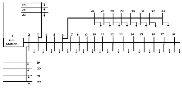
IEEE 33-bus system:

Fig. 1: Single line diagram of 33-bus system

Single line diagram of 33-bus system shown in Fig 1.

581 | P a g e

Before compensation i.e., with no capacitors installed in Radial network, the kW loss is obtained as 205 kW.

The annual cost incurred for 205 kW is calculated as $34,440.

Table 3 Results of 33-bus system

Items Un-compensated Compensated

Total Losses in KW 205.41 160.37

% Loss Reduction - 21%

Candidate buses for

capacitor placement

- 30, 8, 12

Optimal capacitor size in

Kvar

- 350, 1050,450

kVAr Total 1850

Annual cost for kW loss (A)

($)

34,440 26,880

Annual capacitor cost (B)

($/kVAr)

0 475.75

Total annual cost ($) (C = A

+ B)

34,440 27,417.7534

Net savings ($) (D =

35442.96 - C)

0 7,023.2466

% Savings (E =

D/35442.96)

0 20%

Using the proposed method, the capacitors of rating 350, 1050 and 450 kVAr are placed at the optimal locations

30, 8 and 12 respectively. The optimal locations are obtained by sensitivity analysis. As a result, the kW loss is

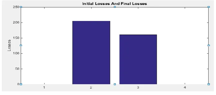
reduced to 160.3691 kW from the base case of 205 kW witnessing a 21% of active power loss reduction as

shown in Fig. 2. The yearly cost incurred for active power loss is calculated as $26,942.003. The amount spent

over the installation of capacitors is been calculated as $475.75.

582 | P a g e

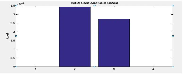
Therefore, the overall annual cost will be the sum of yearly cost of kW loss and the annual cost of capacitor

installed at optimal candidate buses. Net savings per year will be $27,417.75 which leads to 20% of net savings

as shown in Fig. 3.

Fig. 2 represents the losses in KW of 33-bus network. On vertical axis losses are defined and on horizontal axis

initial losses and final losses are defined.

Fig. 3 cost for 33-bus system before and after compensation

Cost of 33-bus system shown in Fig 3. Vertical axis defines cost in $ and horizontal axis defines initial cost

before compensation and final cost which is calculated with GSA.

VI.

CONCLUSION

Thework has been carried out for identification of locations of capacitor to be placed and their size depending

upon the requirement of reactive power. At first analysis has been implemented using sensitive analysis method

to identify the buses which needs the capacitors most. In second step, GSA has been implemented to find out the

size of capacitors. Coding scheme has been developed for above mentioned two steps. The methodology has

been implemented for 33 – Bus system and 141 – Bus system. Following conclusions are drawn from the study.

1. The compensation is provided to minimize the losses.

2. The compensation is bearing in to the maximization of annual savings of cost of power losses.

3. The algorithm is effective in deciding capacitor placement and size of capacitors for different number of

busses and for different sizes of capacitors

VII.

FUTURE

SCOPE

1. The work has been carried out for 33 bus system in distribution system. This allocation of capacitors can be

extended to other bus system in distribution system.

2. For load flow analysis Evolutionary Computation Method can be used.

VIII.

APPENDIX

A.

NOMENCLATURE

Kp equivalent annual cost of power loss in $/(kW-year)

kcfc cost of capacitor spent for one unit of kVAr (Cost/kVAr) or annual capacitor installation cost.

583 | P a g e

Maj active gravitational mass related to agent j.

Mpi passive gravitational mass related to agent i.

G(t) gravitational constant at time t, e is a small constant.

Rij(t) Euclidian distance between two agents i and j.

REFERENCES

[1] Shuaib Y.Mohamed, M. Srya Kalavathi and C.Christober Asir Rajan. ”Optimal capacitor placement in

radial distribution system using Gravitational Search Algorithm”, Electrical Power and Energy Systems,

Vol. 64, 2015, pp 384–397.

[2] Devabalaji K.R., K. Ravi and D.P. Kothari, “Optimal location and sizing of capacitor placement in radial

distribution system using Bacterial Foraging Optimization Algorithm”, Electrical Power and Energy

Systems, Vol. 71, 2015, pp 383–390.

[3] Sabri Norlina Mohd, Mazidah Puteh, and Mohamad Rusop Mahmood, “A Review of Gravitational Search

Algorithm”, International Journal Advance Soft Computer Applications, Vol. 5, No. 3, Nov 2013, pp

2074-8523.

[4] Shaw Binod, V. Mukherjee and S.P. Ghoshal, “A novel opposition-based gravitational search algorithm for

combined economic and emission dispatch problems of power systems”, Electrical Power and Energy

Systems, Vol.35, 2012, pp 21–33.

[5] Khajehzadeh Mohammad and Mahdiyeh Eslami, ”Gravitational search algorithm for optimization of

retaining structures”, Indian Journal of Science and Technology Vol. 5 No. 1, jan 2012, pp 0974- 6846.

[6] Rao R. Srinivasas, S.V.L. Narasimham and M. Ramalingaraju, “Optimal capacitor placement in a radial

distribution system using Plant Growth Simulation Algorithm”, Electrical Power and Energy Systems,

Vol.33, 2011, pp 1133–1139.

[7] Huang Yann-Chang, Yang Hong-Tzer,” Solving the capacitor placement problem in a radial distribution

system using Tabu search approach”, IEEE Trans Power Delivery, Vol.11, No. 4, 1996, pp 1868–73.

[8] Venkatesh B, Ranjan R,”Data structure for radial distribution system load flow analysis”, IEEE

Proc-Generation, Transmission Distribution, 2003, pp 150-10.

[9] Rashedi Esmat, Hossein Nezambadi-Pour and Saeid Saryazdi,”GSA: A Gravitational Search Algorithm”,

Information Sciences, Vol.179, 2009, pp 2232–2248.

[10] Hsiao Ying-Tung, Chen Chia-Hong, Chien Cheng-Chih,”Optimal capacitor placement in distribution

systems using a combination fuzzy-GA metho”,Elsevier International Journal Electrical Power & Energy