A genetic algorithm for designing optimal patch configurations in GIS
by Christopher J Brookes, MSc.
A thesis submitted for the degree of Doctor of Philosophy
University College University of London
Abstract
Geographical Information Systems (GIS) are used for several types of spatial planning but so far they have not been used for optimal patch design. Optimal patch design is a generic spatial problem in which the objective is to design spatially explicit landuse maps when both the composition and configuration of patches are important criteria. There are many applications in conservation, forestry management, watershed management and the management of large military estates.
This thesis describes a new autonomous computer program, the genetic algorithm for optimal patch design (GAPD). GAPD combines four components: a genetic search algorithm, a parameterised region growing (PRG) program, raster GIS measurement functions and multi-criteria decision-making methods. The key component is the PRG which translates between the aspatial domain of the search algorithm and the spatial domain of the GIS. GAPD generates landuse maps that optimise the configuration and composition of patches to meet multiple objectives for a given set of input maps and criteria.
The theories of landscape ecology are used to establish a framework for formulating optimal patch design problems. The thesis describes the conceptual design ofGAPD and its implementation and test, first as a prototype for solving single patch problems and then as a fully functional system for solving multi-objective multi-patch problems. The feasibility of GAPD was established by investigations of issues concerning the representation and measurement of configuration in raster data structures and by testing the efficiency and effectiveness of GAPD with simple problems. GAPD was further evaluated in five hypothetical problems designed to cover a range of different scenarios. The results are promising and show that GAPD has potential as a decision support tool.
Acknowledgements
I am very grateful to Peter Fisher, who set me on the research trail at Leicester University, and to my supervisor at UCL, Paul Denshani, who prevented me from straying from the path. I also thank the Graduate School and the Geography Department of UCL for their financial support and the Geography Department of Portsmouth University for supporting my attendance at conferences.
List of Contents
1.INTRODUCTION, BACKGROUND AND RESEARCH OUTLINE . 18
1.1 Introduction ...18
1.1.1 The Optimal Patch Design Problem ...18
1.1.2 Applications ...18
1.2 Background ...20
1.2.1 Context ...20
1.2.2 Previous research ...22
1.3 Research outline ...23
1.3.1 The research question ...23
1.3.2 Aims and Objectives ...24
1.4 Implementation and test ...24
1.4.1 Conceptual model ...24
1.4.2 Implementation ...25
1.4.3 Testing ...26
1.5 Structure of the thesis ...27
1.6Sunimary ...28
2. DECISION-MAMNG ...29
2.1 Introduction ...29
2.2 Overview of decision science ...29
2.3 Multi-Criteria Decision-Making ...32
2.3.1 Overview ...32
2.3.2 Compensatory methods ...33
2.3.3 Non-compensatory methods ...36
2.4 Search methods ...37
2.5 Decision-making and decision support in GIS: A review ...40
2.6 Summary ...43
3. OPTIMAL PATCH DESIGN AND CONSERVATION ...44
3.1 Introduction ...44
3.2 Ecological background ...44
3.2.1 The fragmentation problem ...44
3.2.2 Conservation strategies and goal setting ...45
3.3 Applications of decision-making techniques to conservation ...47
3.4 Reserve Design - designing optimal patches ...48
3.4.1 Composition and configuration ...48
3.4.2 Spatial factors ...48
3.4.2.1 Landscape ecology ...49
3.4.2.2 Conservation biology ...51
3.4.3 Summary of spatial influences ... 55
3.5 Summary ...57
4. OPTIMAL PATCH DESIGN ON RASTER MAPS 59 4.1 Introduction ... 59
4.3 Cell suitability assessment . 62
4.4 Heuristics ... 63
4.4.1 The Iterative Relaxation heuristic ... 64
4.4.2 Region-growing heuristics ... 65
4.5 Search ... 66
4.5.1 Measuring spatial properties ... 67
4.5.2 Evaluating patch utility ... 69
4.6 Overview of the GAPD conceptual design ... 69
5. GENETIC ALGORITIIMS ... 72
5.1 Introduction ... 72
5.2 History and background ... 72
5.3 Genetic Algorithm Fundamentals ... 74
5.4 The canonical genetic algorithm ... 77
5.5 Genetic Algorithms for decision-making ... 77
5.5.1 How genetic algorithms are applied in decision-making 77 5.5.2 When genetic algorithms are applied in decision-making 79 5.6 Review of some genetic algorithm applications ... 80
5.7 Summary of Operational issues ... 82
5.7.1 Coding ... 82
5:7.2 Fitness function ... 82
5.7.3 Genetic Operators ... 83
5.7.4 Initial population generation ... 83
5.7.5 Number of generations ... 84
5.7.6 Selection methods ... 84
5.7.7 Hybrid algorithms ... 85
5.8 Application of genetic algorithms to optimal patch design ... 86
6. DESIGN AND IMPLEMENTATION ... 88
6.1 Introduction ... 88
6.2 GAPD structure ... 89
6.3 The prototype GAPD ... 92
6.3.1 Introduction ... 92
6.3.2 The PRG component ... 93
6.3.2.1 Simple region-growing - SRG ... 94
6.3.2.2 Parameterised shape-growing - PSG ... 95
6.3.2.3 PRG - the fusion of SRG and PSG ... 103
6.3.2.4 Summary ... 106
6.3.3 The prototype genetic search driver ... 106
6.3.3.1 Physical components ... 106
6.3.3.2 Operational context ... 111
6.4 The transition from the prototype to GAPD ... 112
6.4.1 Introduction ... 112
6.4.2 Possible alternative drivers ... 112
6.4.2.1 Variable length string ... 112
6.4.2.2 Hierarchic structure ... 113
6.4.2.4 Why this line was abandoned . 114
6.5 The full function GAPD ... 115
6.5.1 Modffied PRG ... 115
6.5.2 The GAPD driver ... 118
6.5.3 Pragmatic variations in the implementation of GAPD ... 119
6.6 The measurement and evaluation functions ... 119
6.6.1 Basic raster functions ... 120
6.6.2 Attribute measurements ... 121
6.6.3 Evaluation functions ... 122
6.7 Further developments ... 124
6.8 Summary ... 125
7. FEASIBILITY TESTS ... 126
7.1 Introduction ... 126
7.2 The issue of shape in rasters ... 126
7.2.1 Introduction ... 126
7.2.2 The raster data structure ... 127
7.2.3 Measuring shape on a raster ... 129
7.2.4 Experiment 1: Effect of measurement technique ... 130
7.2.5 Experiment 2 Varying the shape control parameters ... 133
7.2.6 Experiment 3 : Effect of size ... 134
7.2.7 Experiment 4 : Effect of shape control parameters ... 136
7.2.8 Conclusions ... 139
7.3 Effectiveness ... 141
7.4 Efficiency ... 143
7.4.1 Introduction ... 143
7.4.2 Test maps ... 144
7.4.3 Method ... 151
7.4.4 Results ... 152
7.4.5 Discussion ... 157
8. EVALUATION TESTS ... 158
8.1 Objectives and methodology ... 158
8.1.1 Objectives ... 158
8.1.2 Test design ... 158
8.1.3 Test methods ... 161
8.1.4 Test verification ... 162
8.2 Evaluation 1: Designing a single compact patch ... 163
8.2.1 Purpose ... 163
8.2.2 Problem description ... 164
8.2.2.1 Objective function ... 164
8.2.2.2 Data ... 164
8.2.3 Method ... 165
8.2.4 Results ... 168
8.2.5 Discussion ... 175
8.3 Evaluation 2 : Single Objective Multi-Patch ... 177
8.3.2 Problem description
. 177
8.3.2.1 Objective function ...177
8.3.2.2 Data ...178
8.3.3 Method ...180
8.3.4 Results ...182
8.3.5
Discussion ...187
8.4 Evaluation 3 Multi-objective single-patch problem ...188
8.4.1 Purpose ...188
8.4.2 Problem description ...189
8.4.2.1 Objective function ...189
8.4.2.2 Data ...192
8.4.3 Method ...192
8.4.4Results ...194
8.4.5 Discussion ...200
8.5 Evaluation 4 Multi-patch problem ...201
8.5.1 Purpose ...201
8.5.2 Problem description ...202
8.5.2.1 Objective function ...202
8.5.2.2 Data ...204
8.5.3 Method ...205
8.5.4Results ...207
8.5.5
Discussion ...214
8.6 Evaluation 5 : Multi-objective multi-patch problem ...216
8.6.1 Purpose ...216
8.6.2 Problem description ...217
8.6.2.1 Objective function ...217
8.6.2.2 Data ...218
8.6.3 Method ...220
8.6.4 Results ...223
8.6.5 Discussion ...235
8.7 Summary ...237
8.7.1 Review ...237
8.7.2 Generality of GAPD ...237
8.7.3 Performance ...238
8.7.4 Implementation ...240
8.7.5 Appropriate use of GAPD ...240
8.7.6 Conclusion ...241
9. REVIEW AND RECOMMENDATIONS FOR FURTHER RESEARCH ... 242
9.1 Summary ...242
9.2 Recommendations for further research ...244
9.3 Integration with GIS ...246
9.4 Other aspects not previously covered ...247
9.5
Contribution ...250
APPENDICES...252
List of tables
3.1 Landscape elements: their functions and spatial characteristics ... 56
4.1 Levels of spatial arrangement ...68
6.1 Comparison of the prototype GAPD and the full function GAPD ...93
6.2 Shape definition codes for figure 6.7 ...102
6.3 Genetic code structure and sample parameter domains (the values for size, row and column depend on the problem and the dimensions of the raster) ...108
7.1 GAPD solutions to optimise core area, edge area and both core and edge area, on auniform raster ...142
7.2 Estimated patch sizes for maps in series 1 and 2 ...145
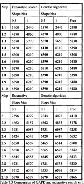
7.3 Comparison of GAPD and exhaustive search in the GAPD efficiency tests.. 153
7.4 Comparison of GAPD and exhaustive search for map 1 in series 2 ... . 156
8.1 Summary of the five evaluation tests ...160
8.la Genetic code for evaluation test 1 ...166
8.2 Genetic algorithm control parameters in evaluation test 1 ...166
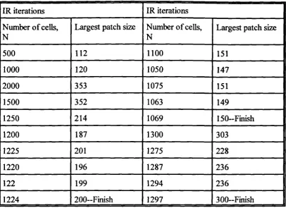
8.3 JR iterations to find a patch of the right size in evaluation test 1 ...168
8.4 Solutions for the three methods in evaluation test 1 ...169
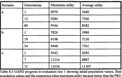
8.5 GAPD progress in evaluation test I showing initial population values, final population values and the generation when maximum utility became better than thePRG solution ...175
8.5a Genetic code for evaluation test 2 ...180
8.6 JR iterations for the 100 and 200 allocations in evaluation test 2 ...183
8.7 The six solutions in evaluation test 2 ...183
8.7a Genetic code for evaluation test 3 ...190
8.9 Patch attribute and utility values in evaluation test 3 ...196
8.10 Change in patch characteristics with changing objective weights in evaluation test 3 ...197
8.10a Genetic code for evaluation test 4 ...206
8.11 Preliminary trial of GAPD with modified PRG for evaluation test 4 ...209
8.12 Comparison of different versions of GAPD in evaluation test 4 ...210
8.13 Comparison of results for different allocation levels in evaluation test 4 ... 211
8.14 Comparison ofdifferent versions ofGAPD for the 600 allocation level in evaluation test4...212
8.15
Conflict between aspatial objectives at different allocation levels in evaluation test5 ...
2208.16 Genetic code for the multi-objective GAPD in evaluation test
5
....
2218.17 Patch attributes for all solutions in evaluation test
5 ...
2248.18 Agriculture patches in evaluation test
5 ...
2258.19 Carpet industry patches in evaluation test
5 ...
2268.20 IR iterations to find the agriculture patch (IR-AG) in evaluation test
5 ....
2278.21 JR iterations to find the carpet industry patch (JR-CARP) in evaluationtest 5 ...227
8.22 PRG parameters (PDCs) for the single objective GAPD solutions in evaluation test5...230
8.23 Utility of the multi-objective GAPD solutions in evaluation test
5
....
2338.24 PRG parameters (PDCs) for the multi-objective GAPD solutions in evaluation test
5 ...
234List of Figures
2.1 A non-monotonic stepwise linear utility function . 34
4.1 GAPD conceptual design ...70
6.1 Logical structure of GAPD ...90
6.2 Physical structure of GAPD ...91
6.3 GAPD flow diagram ...91
6.4 SRG parameter structure (PDC) ... 95
6.5 PSG parameter structure (PDC) ...97
6.6 Sinusoidal shape with 4 axes and a ratio of major to minor axes of 2:1 ...98
6.6a Diagram showing the meanings of the measurements d and 0 in equations 6.1 and 6.2 and how they are calculated ...100
6.7 Shapes grown by PSG with dual shape definition codes (the SDCs are listed in table6.2) ...103
6.8 PRG parameter structure (PDC) ...104
6.9 Genetic code for the GAPD prototype ...107
6.10 Genetic operators (a): crossover, mutation and creep ...109
6.11 Genetic operators (b): average and sum ...110
6.12 Genetic code for the full function GAPD ...116
6.13 Core area and edge area for various shapes ...122
7.1 Variation of core area score with size ...131
7.2 Variation of P1 score with size ...132
7.3 Variation of core area with number of axes for 3 numerator values ...134
7.4 Variation of core area with size for a constant proportional edge effect .... 135
7.5 Variation of core area with size for number of axes = 8 ...137
7.7 Variation of core area with size for number of axes = 12 . 138 7.8 Shapes found by GAPD optimising core (top row), edge (bottom row) and both core
andedge (middle row) ...143
7.9 Suitability map 2.1 ...146
7.10 Suitabilitymap2.2 ...146
7.11 Suitabilitymap2.3 ...147
7.12 Suitability map 2.4 ...147
7.13 Suitability map
2.5 ...
1487.14 Suitabilitymap2.6 ...148
7.15 Suitability map 2.7 ...149
7.16 Suitability map 2.8 ...149
7.17 Suitabilitymap2.9 ...150
7.l8Suitabilitymap2.10 ...150
7.19 GAPD and exhaustive search utility scores in map series 1 ...154
7.20 GAPD and exhaustive search utility scores in map series 2 ...154
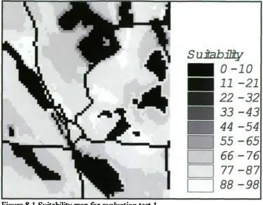
8.1 Suitability map for evaluation test 1 ...165
8.2 Patch found by IR for the 150 allocation in evaluation test 1 ...170
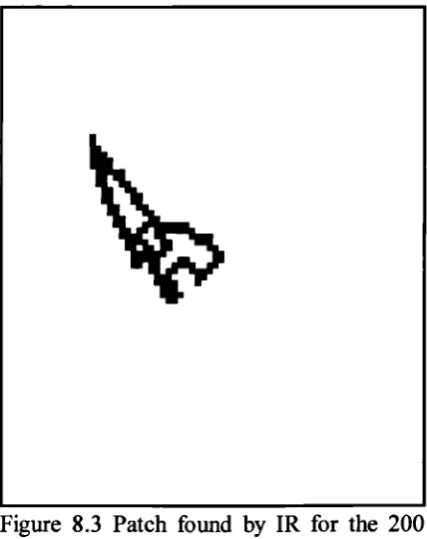
8.3 Patch found by IR for the 200 allocation in evaluation test 1 ...170
8.4 Patch found by IR for the 300 allocation in evaluation test 1 ...171
8.5
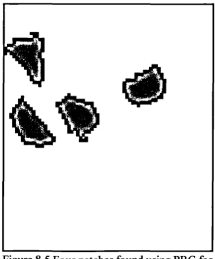
Four patches found using PRG for the 150 allocation in evaluation test 1 ... 1718.6 Four patches found using PRG for the 200 allocation in evaluation test 1 ... 172
8.7 Four patches found using PRG for the 300 allocation in evaluation test 1 ... 172
8.8 Patch found by GAPD for the 150 allocation level in evaluation test 1 ...173
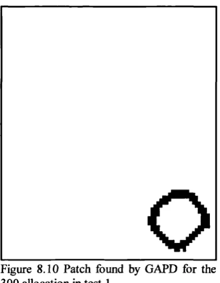
8.10 Patch found by GAPD for the 300 allocation level in evaluation test I .... 174
8.11 Suitability map for evaluation tests 2 and 3 ...179
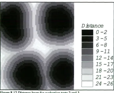
8.12 Distance layer for evaluation tests 2 and 3 ...179
8.13 JR-al: patches found by JR for the 100 allocation in evaluation test 2 ...184
8.14 JR-a2: patches found by JR for the 200 allocation in evaluation test 2 ...184
8.15 G-al: patches found by GAPD for the 100 allocation in evaluation test 2, with no distanceconstraint ...185
8.16 G-bl: patches found by GAPD for the 100 allocation in evaluation test 2, with a distanceconstraint ...185
8.17 G-a2: patches found by GAPD for the 200 allocation in evaluation test 2, with no distanceconstraint ...186
8.18 G-b2: patches found by GAPD for the 200 allocation in evaluation test 2, with a distanceconstraint ...186
8.19 Optimal patch for the core objective (weight 10-0) in evaluation test 3 .... 198
8.20 Optimal patch for two equally weighted objectives (weight 5-5) in evaluation test 3 ...198
8.21 Optimal patch for the isolation objective (weight 0-10) in evaluation test 3. 199 8.22 Data layer showing landuse categories in evaluation test 4 ...213
8.23 Six patches found by iterative application of single patch GAPD in evaluation test 4 ...213
8.24 Six patches found by fixed multi-patch GAPD in evaluation test 4 ...214
8.25 Eight patches found by variable multi-patch GAPD in evaluation test 4 ... 214
8.26 Suitability map for agriculture in evaluation test 5 ... 219
8.27 Suitability map for the carpet industry in evaluation test 5 ... 219
8.28 Location of the agriculture patch found by JR in evaluation test 5 ... . 228
8.30 Location of the agriculture patch found by single objective GAPD in evaluation test5...230 8.31 Location of the carpet industry patch found by single objective GAPD in evaluation test5...231 8.32 Location of the agriculture and carpet industry patches found by the hierarchical
GAPDmethod in evaluation test 5 ... 232
List of Appendices
APPENDIX I. Technical programming notes. 252 APPENDIXII. Pseudo code ... 255
Additional material
Definitions 1. Acronyms
GAPD. Genetic algorithm for optimal patch design GIS. Geographical Information System
MCDM. Multi-criteria decision-making MPDC. Multiple patch definition code PDC. Patch definition code
PRG. Parameterised region-growing PSG. Parameterised shape-growing SRG. Simple region-growing SDC. Shape definition code
2. IDRIS1 functions
AREA. Calculates the total area of each cell type. Note that if two patches have the same type the AREA command will return the total area of both patches, not the area of each patch.
EXTRACT. Extracts values from one image using features defined on an overlay image.
GROUP. Groups contiguous cells with the same value into patches and assigns a patch identifier to each cell in the group. GROUP and AREA can be used together to find the area of each patch.
HISTO. Displays statistical information about an image, such as the number of cells of each type.
OVERLAY. Includes several options for overlay processing including mathematical operations. If an image is multiplied by a binary image zero valued cells in the binary image produce zero valued cells in the output image, therefore overlay can be used as a masking operation.
RECLASS. Classifies cells by their value and assigns a new value to each cell. STRETCH. Transforms an image by reassigning the maximum and minimum values and then recIassiI,ring each intermediate cell using an interpolation procedure. The interpolation can be linear or statistical. Stretch is typically used to improve the visual appearances of images.
3. IDRISI file structures
Document file. IDRISI images are held in two files. The document file is a text file containing a description of the image. It includes information such as the dimensions of the image and the range of cell values.
Image file. The image file holds the actual cell values. Image ifies can only be processed correctly if they are accompanied by a document file.
4. Other terms
Boundary effects. Effects caused by the finite limits of rasters. A patch cannot grow outside the raster so patch shape is constrained near the raster boundary.
Composition. The amount of different patches or elements within patches. Configuration. The spatial distribution and shape of patches.
Core area. The inner area of a patch not affected by edge effects. Where edge effects are strong the core area is much smaller than total patch area.
Edge effects. Ecological, and other, effects occurring at the edge of patches. Edge effects create a transition zone between the interior and exterior of patches.
Effectiveness (of a search procedure). A measure of the quality of the solutions. A search is effective if it finds good solutions.
Efficiency (of a search procedure). A measure of the quality of the process. A search is efficient if it finds good solutions with limited resources. More rigorously, efficiency is the ratio of the alternatives examined to the total number of alternatives in the search space.
1. INTRODUCTION, BACKGROUND AND RESEARCH OUTLINE
1.1 Introduction
Optimal patch design is a generic spatial planning problem because pattern and process are intricately linked in many spatial systems. The relevance of configuration as a criterion has been recognised within different planning contexts but the treatment of spatial factors has been ad hoc. This research addresses the issues in optimal patch design, formulates a conceptual model for a generic decision support tool, identifies suitable components and implements the model as a working system.
A major part of this thesis is the development and test of a computer system for designing optimal patch configurations using raster GIS. Some work has been carried out recently on similar continuous space problems with vector systems (Krzanowski
1997). The Genetic Algorithm for optimal Patch Design, GAPD, generates raster maps showing the explicit location and configuration of patches. The composition and configuration of patches are optiniised to meet multiple objectives subject to multiple criteria. GAPD links a genetic algorithm with raster GIS and multi-criteria decision-making routines. A novel technique, parameterised region-growing, PRG (Brookes, 1 997a), is used as a bridge between the aspatial domain of the genetic algorithm and the spatial domain of the GIS.
1.1.1 The optima/patch design problem
patches, and spatial relationships among patches. Patch is a term used in landscape ecology to denote physical entities. Patches can also be human constructs such as administration districts, planning zones or catchment areas. In the development and test of the methodology this research concentrates on problems in which spatial extent, configuration and distribution are significant criteria, because these are the areas that have not been addressed previously. However, the research has wider significance because such problems can be seen as existing somewhere in the middle range of a spectrum of problems. At one extreme, the objective is to partition a whole space and at the other to locate multiple point sites (ie. isolated cell). In the latter case, although the sites themselves are not patches, they implicitly define patches if the pattern of sites and, therefore, the configuration of the space between sites, is significant. Thus, a generic methodology for addressing optimal patch design is relevant to a range of site location and landuse planning problems.
1.1.2 Applications
important to avoid suspicion of gerrymandering. When locating facilities at sites the catchment may need to include divers social elements. Configuration can affect physical systems in various ways. The distribution of landcover patches in a watershed will affect runoff and consequently erosion, sedimentation and flooding. Forests are managed for efficient timber production, for which large uniform stands are advantageous, and conservation and recreation which require a pattern of smaller more diverse stands. The spread of forest fires are also affected by planting patterns.
1.2 Background
1.2.1 Context
The idea that pattern and process are interrelated is common to many spatial disciplines and it is fundamental in landscape ecology. Landscape ecology is the study of kmdscape processes and landscape structure (Forman & Godron, 1986). The contribution of landscape ecology in this research is to provide a set of concepts for formulating optimal patch design problems. Patch is a term used in landscape ecology to denote spatial units in a landscape. Configuration refers to the shape and spatial distribution of patches. Composition is the amount of different elements within a patch or landscape.
Landscape ecology is holistic and the links between form and process are implicit and hard to quantiQy. In other disciplines the link is clearer. Many natural processes are influenced by both the composition and configuration of patches. Consequently, alternative configurations have different value with respect to particular objectives and criteria. For example patch configuration affects:
• ecological functions and the value of habitats;
• surface flow routing in watersheds and catcbments with implications for erosion and flooding;
• the spread of fires; and
In part, the motivation for this research comes from an interest in conservation and that is why conservation biology was chosen to exemplify the effects of configuration on value. Ecologists have studied the effects of spatial factors on habitat quality and have been able to draw up guidelines for the design of nature reserves (Smith & Theberge, 1986; Morrison et a!., 1992). These guidelines can be translated into evaluation functions within a decision-making context. Analogous ideas can be used in other contexts, as outlined in above (1.1.2).
Optimal patch design is a type of landuse planning problem. In landuse planning many of the relevant attributes such as vegetation, slope, soil type and so on, vary continuously over space. This spatial variability is better handled using raster data structures than vector. Raster GIS functions are perfectly adequate for the suitability assessment that this type of problem demands (Eastman et a!., 1993; Pereira & Duckstein, 1993; Jankowski, 1995). If configuration is irrelevant then suitability analysis is sufficient. However, when configuration is relevant the problem is more complex and other methods are needed.
GIS do not have the functionality for what Tomlin calls prescriptive modelling with holistic criteria (Tomlin, 1990). Holistic criteria, as opposed to atomic criteria, can only be evaluated when the solution is known. In this thesis the terms dynamic and static criteria are used instead of holistic and atomic respectively because they express this fundamental difference better. Tomlin's solution is to use ad hoc heuristics. He proposes some example problems and heuristics that can be implemented in GIS. An alternative approach is to use GIS as a support tool, coupled with other tools in an interactive decision-making environment (Fedorowick, 1993; Barrett & Peles, 1994; Chuvieco, 1993). GAPD is a single, autonomous system that handles the data, criteria and objectives pertinent to optimal patch design.
spatial criteria are the location of points and the connections between them. The difference between optimal patch design and these other types of problems is that the spatial entities, the patches, have a spatial extent and, therefore, an explicit shape as well as a location.
A number of computational techniques have been developed which exploit the power of digital computers. These techniques are now being used in GIS and image processing applications (Openshaw & Abrahart, 1996). Of most relevance to optimal patch design are genetic algorithms which are powerful generic search methods for finding solutions to complex problems. The main problem with their application to optimal patch design is to find suitable data structures that represent two dimensional entities and at the same time are amenable to manipulation by the genetic algorithm.
Decision-making systems require data. Developments in remote sensing technology, both in sensor hardware and image processing software, mean that the necessary data for landuse planning can be acquired in sufficient quantity, detail and with regular updates.
1.2.2 Previous research
1.3 Research outline
1.3.1 The research question
In optimal patch design the objective is to produce spatially explicit landuse plans that optimise both the configuration and composition of patches. Optimal patch design is a complex spatial problem. A number of key features require particular attention.
• The attributes that contribute to patch composition are distributed spatially. They vary continuously and, consequently, are best represented in raster data structures.
• Patch configuration is a spatial property whose measurement is greatly facilitated by the use of GIS which should therefore be integrated within the chosen methodology. • Patches are evaluated against multiple criteria.
• Some criteria are static: a single evaluation applies to all possible solutions. Criteria relating to composition are mainly static.
• Some criteria are dynamic: they must be re-evaluated for each alternative solution. Criteria relating to configuration are dynamic.
• Spatial decisions frequently involve multiple conflicting objectives.
• There are an infinite number of possible patch configurations and subtle changes in patch location or configuration can have disproportionate effects on utility. Thus, the size and complexity of the search space demands an efficient search mechanism. • Most aspects of spatial decision-making involve uncertainty. There is not only uncertainty in the attribute measurements but also in the criteria and objectives.
1.3.2 Aims and Objectives
The principal objective of the research is to build and test an autonomous computer system for the design of optimal patch configurations. A secondary objective is to link GAPD with GIS and consider alternative ways of achieving this. The end product, GAPD, will be evaluated against the following considerations:
• The patches generated by GAPD must show that GAPD responds to different criteria and different objectives.
• The patch configurations should look right. For example, in simple problems it may be obvious that patches should be compact.
• GAPD must be useable and flexible. It must be adaptable to different problem types. • GAPD must be efficient: it must make better use of computer resources than an exhaustive search.
• GAPD must be effective. The solutions should be better than random guesses.
Working toward these goals will involve developing an understanding of the nature of the optimal patch design problem and the limitations of the system.
1.4 Implementation and test
The research strategy is to:
1. Produce a conceptual system design.
2. Develop an appropriate spatial search mechanism.
3. Implement the system in a suitable programming language. 4. Evaluate the system using realistic data and problems.
1.4.1 Conceptual model
a genetic algorithm: genetic algorithms are capable of efficiently exploring complex decision spaces. Measurement and evaluation are performed by raster GIS functions, that measure patch attributes, and MCDM methods, that convert attribute values to utility scores. These three components employ conventional techniques. The translation function is performed by parameterised region-growing (PRG): PRG serves as a bridge to link existing techniques in a single autonomous system. No single component of GAPD is adequate in itself but GAPD exploits the advantages of each.
The potential problem with search is that generic search algorithms, such as genetic algorithms, are aspatial and operate on internal data structures, typically strings. Patch structure is spatial and evaluation functions operate on raster maps. A code is needed to translate between structures used by the search algorithm and the spatial representation of patches. PRG provides the link: the PRG algorithm grows patches on a raster map under the control ofa string of numeric parameters. The parameter strings are easily incorporated into a genetic algorithm and the raster maps are in a suitable format for GIS operations. Thus, PRG translates from string structures in the search domain to spatial structures in the problem domain.
GAPD addresses the main problem in optimal patch design - the handling of dynamic criteria. It explicitly evaluates dynamic criteria for each alternative patch configuration. Methods that explicitly evaluate atomic criteria only, rely on ad hoc problem-specific heuristics. GAPD uses a universal search heuristic that is independent of the problem domain. Only the criteria and objectives, and hence the measurement and evaluation functions, are problem specific. Another feature of GAPD is that it can operate directly on multiple data layers and, therefore, goes beyond traditional suitability mapping.
1.4.2 Implementation
can be used as a translation function within a search algorithm it must be able to generate all possible patches. The first step in the implementation of GAPD was to improve the original PRG algorithm to grow a wider range of shapes.
The translation component dictates the form of the genetic code used in the genetic algorithm. Basic genetic algorithm source code is in the public domain: a version published by Ribeiro Filho et al. (1994) was adapted and extensively modified. Genetic algorithms are conceptually simple and of proven value in solving complex, non-linear problems (Goldberg, 1989; Davis, 1991) but the application of genetic algorithms to specific real world problems is non-trivial.
The measurement and evaluation components consist of a number of problem specific routines. The utility functions are based on two theoretical models taken from the conservation biology literature. The models use simple concepts and are simple to implement - hence they run quickly and are easy to debug. In the core area model, patch shape has a large effect on patch utility (Laurance, 1991); and in the minimum cumulative resistance model, both shape and position relative to other patches are important (Knaapen et al., 1992).
GAPD was implemented as a series of linked functions coded in the C programming language (Schildt, 1991). GAPD was initially programmed to run on a micro-computer (i.e. a PC) and, with minor modifications, was later converted to run on a UNIX workstation. GIS raster functions for patch analysis were coded in C as part of GAPD. GAPD is loosely coupled with the IDRISI GIS which is used to produce geographic datasets for input to GAPD and for display and further analysis of the outputs.
1.4.3 Testing
in raster data structures. Further tests looked at the representational power of the PRG algorithm and the efficiency of the genetic search driver.
GAPD was further evaluated by testing against a number of artificial trial problems of varying complexity. Although the complexity of a problem is not strictly quantifiable high spatial variability in the data, complex or compound utility functions and multiple patch solutions are characteristics of complex problems. Simple problems have low spatial variability, simple utility functions and are constrained to have single-patch solutions. Four broad types of problem are identified:
• Single patch-single objective (SPSO); • Single patch-multiple objective (SPMO); • Multiple patch-single objective (MPSO); and • Multiple patch-multiple objective (MPMO).
To give some idea of the efficiency and effectiveness of the system, the results of the trials were compared with results that were obtained using other heuristics. Results were also evaluated by considering the size of the search space and by estimating upper bounds to the solutions.
1.5 Structure of the thesis
The conventional components of GAPD are discussed in the opening chapters. Chapter 2 deals with multi-criteria decision-making and search. Chapter 3 is a review of landscape ecology and conservation biology. Chapter 4 reviews some applications of GIS to decision-making and sets out the optimal patch design problem. Genetic algorithms are dealt with in Chapter 5.
GAPD was tested in two phases. Feasibility testing of the GAPD concept is described in Chapter 7. The second phase, the evaluation tests, are described in Chapter 8. Five hypothetical problems, using real datasets, were designed to test the effectiveness and efficiency of GAPD in a range of situations. The ffllh test is a variation on a case study in Kathmandu originally done by Eastman et al. of the IDRISI project (1993).
The final chapter summarises the achievements of the research and sets out an agenda for further work.
1.6 Summary
Designing optimal patches in raster GIS is a complex problem because the size and shape of patches and the spatial relations among them are all criteria. When landuse planning can be done without regard to the composition and configuration of patches the conventional decision-making methods can be applied because there are no dynamic criteria. Suitability analysis using GIS is sufficient because each cell is a viable alternative and the problem is simply a matter of scoring each cell. This is no longer the case when configuration is relevant. In the simplest case there will be a constraint on minimum patch size and individual cells are no longer viable alternatives. Instead, the viable alternatives are patches or clusters of cells.
2. DECISION-MAKING
2.1 Introduction
This chapter is an overview of decision-making methods particularly those which are relevant to the design ofpatch configurations. Optimal patch design is a complex spatial problem involving the integration of numerous spatial and aspatial criteria. There are an infinite number of possible patch configurations and the key issue in decision-making terms is the generation of good alternative candidate solutions. An efficient search method is needed to address this aspect of the problem. Conventional multi-criteria decision-making methods can be applied to evaluate alternative solutions and choose between them, thus driving the generation process. The spatial nature of the problem demands the use of raster GIS and this chapter also includes a review of some of the ways GIS are used for decision support.
In conservation applications, patches designed by decision makers must be realised through management practice, for example periodic felling, restoration of vegetation, fencing off to prevent grazing and so on. Chapter 3 says more about how patches as design artefacts relate to and differ from physical patches resulting from natural ecological processes. The special nature of optimal patch design as a spatial problem is set out more thoroughly in Chapter 4.
2.2 Overview of decision science
developing, implementing and evaluating a methodology for designing optimal patch configurations.
Early decision-making techniques were developed to address logistical and economic problems and were highly deterministic (Wagner, 1972). With the help of fast digital computers, decision science is now applied to a broader range of situations. The problems tackled have become more complex and decision-making tools are now more varied and less deterministic (Minch & Sanders, 1986). Computer packages for decision-making are now integrated in decision support systems that allow a more flexible, exploratory approach to decision-making (Densham, 1991). The range of spatial problems that are addressed using formal methods and GIS includes site location, optimal routing, location-allocation and suitability assessment. Many aspects of spatial decision-making using a combination of GIS and formal decision-making methods are discussed in great detail in the literature (Jankowski, 1995; Pereira & Duckstein, 1993; Carver, 1991; Eastman
etal.,
1995).Complex decision problems are characterised by multiple incompatible criteria, multiple conflicting objectives and uncertainty. A well-structured problem is one that always yields the same result whereas in a loosely-structured problem the result will vary depending on the people solving the problem, because of their assumptions, values and judgements, and on the methods used (Minch & Sanders, 1986). In such cases there is no single best solution and in some situations it may be sufficient to find a satisflictory solution instead of a global optimum. There are other factors to consider in choosing a solution method particularly the time and resources available. In real applications as opposed to theoretical situations these are important pragmatic and practical considerations.
At the operational level all decision-making methods involve three steps: • identification of alternatives
• evaluation of alternatives
Decision science has produced many multi-criteria decision-making (MCDM) methods to evaluate and compare alternatives. When there are large numbers of alternatives search techniques are used to identil' promising alternatives. Efficient search techniques rely on feedback information about the relative value ofalternatives. MCDM and search methods are discussed more fully in subsequent sections.
Before discussing techniques in detail certain other issues must be mentioned. Risk and uncertainty are important considerations in any decision-making context. There is uncertainty in the physical attribute measurements, the evaluation functions that convert measurements to scores, the relative weighting or ranking of criteria and possibly also in the objectives. Certain methods make an assumption that criteria are independent and when this is not valid there is added uncertainty. If the criteria are not independent there will be epistatic or non-linear effects that magnify the uncertainty because small changes in attributes can generate disproportionately large changes in resultant utility (Goldberg, 1989). Finally, there are temporal considerations. Most decisions have consequences and dependencies that extend into the future. For example, when deciding where to locate a nature reserve the decision may be influenced by predictions of climate change and about future landuse requirements, which are important because nature reserves are long term features. Consequently there is uncertainty in the final decision and, therefore, a risk that the decision is not actually the best.
Methods for dealing with risk and uncertainty include techniques using probability (Goodchild et al., 1992), fuzzy sets (Letmg, 1988; Burrough, 1989; Burrough & Heuvelinck, 1992; Van Gaans & Burrough, 1993) and artificial inteffigence (Chen et al.,
1994). However, these are all limited because they ultimately rely on subjective judgement. Perhaps the best way to handle uncertainty is within a decision support
Densham, 1993).
This thesis is not concerned directly with uncertainty issues except to say that the operational context of any decision support tool such as GAPD must be considered.
2.3 Multi-Criteria Decision-Making
2.3.1 Overview
The terminology in the literature is not always consistent and in the context of this thesis MCDM is used to embrace all techniques designed to handle situations with multiple criteria or multiple objectives. Other related terms used in the literature are multi-criteria evaluation, multi-objective programming and goal programming. These terms are not synonymous and a single term is used here for simplicity. Essentially MCDM is about the evaluation and comparison of disparate entities.
In MCDM the problem is how to compare alternatives based on seemingly incompatible criteria. Since any method of comparing alternatives inevitably involves arbitrary judgements, all methods are open to criticism. However, formal methods provide a
framework for decision-making which can be useful in justifying decisions as well as aiding the decision-making process. Such a framework gives a structure, a degree of repeatability, and breaks the problem into components where arbitrary judgements are easier to make because they involve a single criterion. Judgements are explicitly stated along with any assumptions, so that the decision can be explained and justffied to interested parties.
to compare alternatives. There are two basic approaches: compensatory methods and non-compensatory methods. The compensatory approach assumes that criteria are compatible and that high scores for one criterion can compensate for low scores against another criterion. Non-compensatory methods do not allow a trade-offbetween criterion scores. Both approaches employ a decision rule to identi1' the best alternative. In both approaches alternatives that do not satisf' constraints, i.e. ones that are infeasible, are eliminated from further consideration.
Multiple objectives add another level of complexity to problems. As with multiple criteria the difficulty lies in the fact that objectives are expressed in different terms. Methods for tackling multi-objective problems are similar to those used for multiple criteria. Objectives can be ranked so that the problem is reduced to a series of single objective problems. Compensatory methods can be used to combine utility scores against individual objectives into a single utility score. Multi-objective decision-making methods are well documented (for example, see Tanuz, 1996).
2.3.2 Compensatory methods
be done by defining a conversion function in consultation with experts. A step-wise function to convert interval scale attribute measurements can be found using the following iterative process from Pereira and Duckstein (1993).
• First, identi!' the attribute values that represent the maximum and minimum utility, and the midpoint between them.
• Second, identily another set of midpoints between the points already defined. • Repeat the second step until the form of the function is sufficiently well defined. A similar process can be used to define conversion flmctions for attributes measured on categorical or ordinal scales. A non-monotonic function can be built up out of linear sections, each of which is derived using the above method. Figure 2.1 shows a non-monotonic stepwise utility function.
Figure 2.1 A non-monotonic stepwise linear utility function.
In raster GIS the most common compensatory method for comparing alternatives employ some kind of weighted summation technique (Jankowski, 1995; Pereira & Duckstein, 1993; Eastman et a!., 1995). One such technique is compromise programming.
from the ideal is a measure of relative suitability for each alternative. Alternatives that violate any constraints are eliminated.
Once the attribute measurements have been standardised, the distance from the ideal point can be calculated by combining the criterion scores into a single score using a weighted combination. Some factors may be more important than others in determining combined suitability, in which case equal distances in suitability space are not equivalent in different dimensions. The relative importance of individual factors is reflected in the weights assigned to them. Determining weights is again problematical and Eastman et a!. (1993) describe a method and a function in the IDRISI GIS (Eastman, 1993), that determines weights based on a series of preference choices.
Taking together the ideas of a utility space, standardised utility scales and relative factor weights, the score S0 of an alternative a, is calculated by equation 2.1. The utility score for factor is X,, for alternative a and X,. for the ideal point. The weights are denoted by W, and there are N factors. The alternative with the minimum score is the winner.
N !
Sa = [ W°.(X -X,0 )" ] Equation 2.1
The weights are normalised so that
WI = 1 Equation 2.2
a perfect trade-off between factors because an increase in distance on one factor can be compensated by an equivalent decrease in another factor. Ifp> 1 then Utility decreases more rapidly with distance, so that large distances are relatively more important. Asp >> 00 then the evaluation approximates to a minimax rule where the suitability of an alternative is only as good as its worst score against all criteria (Pereira & Duckstein,
1993). Pereira and Duckstein (1993) found thatp=1O was high enough to be effectively co. Often the scale is such that the optimal score is 0 and the worst score is 1.
In ideal point analysis, the alternative with the smallest score is the winner. A mathematically equivalent technique simply takes a weighted combination of standard scores to derive a single overall score for each alternative. The alternative with the highest score is the solution. This method is called weighted summation.
An alternative compromise technique is Concordance-Discordance analysis (Carver, 1991). This method performs a pairwise comparison of each alternative against all the others to derive a dominance ranking for each alternative. The concordance measures the degree to which one alternative is superior to another for each criterion and the discordance measures the degree to which it is inferior. By combining the concordance and discordance scores for all criteria each alternative is given an overall ranking. The highest ranking alternative is the optimal solution. Because of the combinatorial explosion, concordance-discordance analysis is sensitive to the number of criteria and alternatives. it is not usually used where there are large numbers of alternatives and for this reason is not recommended for use in connection with raster GIS (Jankowski, 1995).
2.3.3 Non-compensatory methods
The lexicographic and hierarchical optimisation methods require that the criteria be ranked in order of importance but do not assign relative weights. They are iterative techniques whereby the most important criteria are used first. In the lexicographic method the highest scoring alternative on the most important criterion is the winner. If there is a tie then all other alternatives are eliminated and the contest continues with the next ranked criterion until there is a winner. In the hierarchical method alternatives are eliminated if they fail to meet the threshold score for the current criterion.
The conjunctive and disjunctive methods also use thresholds but without ranking criteria. An alternative is eliminated if it fails to meet the threshold on a single criterion (conjunctive) or on all criteria (disjunctive).
The Dominance method also treats each criterion as equal. An alternative, A, dominates another alternative, B, if A scores at least as highly as B on all criteria and higher than B on at least one criterion. B is then dominated by A and is a dominated alternative. All dominated alternatives are eliminated and the non-dominated alternative is the winner. It may be that there is no solution using the dominance method since there may be more than one non-dominated alternative.
In general non-compensatory methods are applicable to problems with relatively few alternatives and these methods often will not identiI' a unique solution.
2.4 Search methods
height values are the utility. Peaks are local optima and the highest peak is the global optimum. Search spaces with many local optima are difficult to solve.
Search methods can be classified according to how they search the decision space. There are four basic methods: enumerative, random, deterministic and heuristic (Goldberg,
1989).
The enumerative method simply visits every point in the decision space and then chooses the best. It is an exhaustive search and is bound to find the optimum eventually. The enumerative method is suitable for problems when there are few alternatives. However, for many search problems it is inefficient and, therefore, impractical.
Random search visits a number of points at random and chooses the best. Random search has no guarantee of finding the best or even of finding anything much better than average. Enumerative and random methods are both blind searches.
Deterministic and heuristic methods make use of some knowledge of the decision space and are useful when the search space has a high degree of regularity, ie. when neighbouring points have more similar utility values than distant points. Using the topographic analogy again, the surface is smooth and continuous not jagged. Deterministic methods partition the search space, discarding segments until only the optimal point is left. Heuristic methods also partition the space but do not guarantee to find the optimal value. There is always a chance that the true optimum has been discarded. For many problems, there are no deterministic methods because the search space is too complex. Heuristic methods are often the only feasible approach.
solution values and the granularity dictates how finely solutions can be distinguished. Thus, the extent and granularity determine how big the space is, that is, how many different possibilities there are. When digital computation is used a theoretically continuous space becomes discrete with a finite granularity. The size of the decision space is an important practical consideration. Complexity is critical when deciding on a solution method because each method works better in different types of decision space.
Many heuristics are based on the hill-climbing concept. Starting with a single guess, for which a utility value is calculated, small changes are made to the guess and the utility is re-evaluated. If the changes improve the solution they are accepted and new changes are tried. This process continues until further changes do not improve the utility. Hill-climbing methods work for fairly simple search spaces but in very complex spaces they are prone to find local optima and get stuck without finding the global optimum.
In recent years a number of new generic search and optimisation methods have been developed. Neural networks (Grossberg, 1988), simulated annealing (Cagan& Mitchell, 1993) and genetic algorithms (Goldberg, 1989) are methods which mimic natural processes within computers. Neural networks mimic the way the brain processes information and they have proved valuable in applications such as pattern recognition. Simulated annealing is analogous to cooling metals to toughen them. Simulated annealing algorithms allow random jumps in the decision space to explore different possibilities. The size of the jumps are slowly decreased so that the algorithm converges on a solution. Genetic algorithms use a universal heuristic based on evolution and natural selection. These methods have all proved superior to conventional methods in some applications because they are able to avoid being trapped by local optima. Genetic algorithms will be discussed more fully in Chapter 5.
operate with feedback which simply ranks two alternatives without giving absolute utility values. The computer system developed in this research project does not use non-compensatory methods but there is no reason in principle why it should not. In the chapter describing the implementation of GAPD it will be seen that a compensatory method fits in more easily with other GAPD components. Alternative implementations of GAPD could equally well use non-compensatory evaluation methods.
2.5 Decision-making and decision support in GIS: A review
GIS can be used for decision-making in two ways, either as decision support systems in their own right, or as auxiliary analysis tools loosely coupled with decision support software. GIS do not have strong decision-making functionality and the loose coupled approach is often used. One advantage of loose coupling is that the GIS is used for spatial analysis, where it is strong, and the output can be fed into a number of different, specialist decision support packages. Thus, MCDM methods which are not easy to implement in GIS, or which are already well supported by existing software, can be used. The most appropriate method rather than the one most convenient to implement in GIS can be chosen.
In a location-allocation problem the objective is to select supply sites from a number of potential sites to serve a number of demand locations. The supply sites must satisfy the total demand and the objective is to minimise the total cost of satisfying the demand. The location-allocation problem can be solved using a network data structure i.e. the supply and demand sites are nodes connected by lines. There are a number of heuristic solution methods (Densham & Rushton, 1992). ARC/INFO includes functions for
location-allocation (Environmental Systems Research Institute, 1992).
In site location the objective is to find the best site according to a number of criteria. Generally, GIS have the functionality to measure the attributes of sites but are lacking in functions for converting attribute values to scores and for applying decision rules to identify the best site. IDRISI, however, has functions for the weighted summation compensatory technique plus modules which help in assigning weights and in assessing risks.
Site location problems usually involve suitability assessment. Suitability assessment uses MCDM techniques to assign a score to each location. The score is a measure of the location's suitability for some purpose. Suitability analysis can be performed using the basic GIS buffering and overlay operations. The IDRISI GIS includes a number of functions that facilitate MCDM. The IDRJSI MCE function is a user friendly interface to an ideal point analysis using weighted overlay. Other routines are available to help users to assign relative weights to different criteria and to handle risk and uncertainty. The routines facilitate suitability assessment but do not apply generally to more complex planning problems. Suitability assessment may be the first step in a patch design problem.
each site is scored against each criteria. The scoring process creates a matrix of rows (sites) and columns (criteria). The matrix elements S, are the normalised weighted utility scores for site i according to criterionj. The utility matrix is input to the FORTRAN program which can perfbrm idea! point analysis, hierarchical optimisation or concordance discordance analysis.
Chuvieco (1993) describes a planning problem where the objective was to determine an optimal land reallocation strategy given constraints on the total amount ofland that could be reallocated. A GIS was used at two points in the analysis. First the GIS was used to identiii the total area of land available. This data was fed into a linear programming software package called QSB that determined how much land should be reallocated. However, the package did not specify which land should be allocated. The GIS was involved again to identify actual locations using simple functions such as distance buffering.
Xiang (1993) has also used GIS with linear programming. In this example there are two conflicting objectives and Xiang uses the technique of mitigation costs, or a penalty function, to convert the problem into a single objective. The linear programming component identifies land parcels and the GIS is used to identify conflicts. The system runs in a DSS context.
2.6 Summary
3. OPTiMAL PATCH DESIGN AND CONSERVATION
3.1 Introduction
GAPD is a computer system and it treats optimal patch design as a problem of locating optimal clusters on raster maps. This chapter looks at real world situations where configuration and composition of spatial units is critical. Conservation biology provides many examples of these types of problems. A key issue in conservation is habitat fragmentation which reduces habitats to isolated patches. The utility of a habitat patch is a function of its composition, its configuration and its context in the landscape. The quality of the habitat at the location is critical but the spatial properties of size and shape, and the spatial interactions with other patches, are also significant. Studies in conservation biology, ecology and landscape ecology have lead to the identification of a number of principles and guidelines for nature reserve design. These guidelines can be translated into formal criteria which can be evaluated using GIS functions and incorporated into a decision support tool.
Most conservation biology and landscape ecology is descriptive rather than prescriptive (Shrader-Frechette & McCoy, 1994). This is natural since there is still a lot of uncertainty surrounding conservation objectives and ecological processes. Where efforts are made to apply formal decision-making techniques to issues such as reserve planning they are essentially aspatial.
3.2 Ecological background
3.2.1 The fragmentation problem
small patches which are surrounded by a matrix of developed land. The consequences of this have not been quantified but there is a widely held belief that many species and habitats are under severe threat.
Much research in ecology shows that in fragmented landscapes, spatial factors affect ecosystem functions in many important ways. Different researchers have identified a number of guidelines concerning the size and shape of reserves and the spatial relationships between them. These guidelines are uncertain, specific to particular species or ecosystems and sensitive to the conservation objective. However, the guidelines can be used as a basis for designing evaluation functions which can be implemented in raster GISs and used in conjunction with decision-making methodologies. There are examples of GIS and decision-making techniques being employed to improve nature reserve selection strategies (Davis et al., 1990; McKenzie eta!., 1989; Margules & Stein, 1989). These methods concentrate on aspatial factors and, in view of the importance of spatial factors, there is a need to develop tools which incorporate spatial factors in nature reserve planning.
3.2.2 Conservation strategies and goal setting
Conservation problems cover a wide range of objectives, strategies and scales, from management of individual species at a small scale to strategies for preserving bio diversity at a global scale. Ecosystems are complex and dynamic; ecosystem functions are modified by spatial and temporal factors. Inevitably, uncertainty surrounds conservation objectives and the means to achieve them.
decreasing the value of otherwise suitable habitat. The main consequences of habitat fragmentation which are detrimental to overall habitat value are the reduction in size of habitat patches such that they are not able to support viable populations, the isolation of patches from each other, and the exposure of habitats to interactions with surrounding areas. Habitat patch size and spatial relationships, both with other patches and with the surroundings, should all be taken into account in evaluating habitat suitability and, hence, in deciding where reserves should be located.
Nature reserves are areas which are set aside for conservation and managed in a particular way. Initially, a nature reserve may be physically indistinct from its surroundings but in many cases the administrative boundaries will correspond to physical boundaries and the reserve will be a recognisably distinct physical unit. Reserves that start out as indistinct from their surrounding are likely to become distinct over time. Reserves can be put into three categories depending on the landscape structure: (1) Selected reserves, (2) Rescued reserves and (3) Restored reserves. In the first category there is more potential habitat than is going to be protected and the planners can select areas to be protected. Other areas will be used for forestry, agriculture, etc., with the result that the selected reserves eventually become isolated. Initially, suitable habitat is the matrix surrounding patches of non-habitat, but once the reserves are designated the situation is reversed. In the second category, the potential habitats are already isolated and there is little choice: habitat is patchy in a contrasting matrix. In the third category, the amount of habitat is less than is needed so areas must be restored. As the restoration takes effect, for example by planting to create woodlands or by removing drainage to recreate wetlands, the contrast between patch and matrix increases and over time the reserve will become a physically distinct patch.
3.3 Applications of decision-making techniques to conservation
Conservation planning is done at the strategic and operational level There are numerous conservation objectives and appropriate strategies (Smith & Theberge, 1986; Usher,
1986; Lomolino, 1994; Leader-Williams eta!., 1990; Game & Peterken, 1984; Theberge, 1989).
Two well-documented reserve selection methodologies, gap analysis and representative reserve selection, are based on the premise that all species should be preserved and, consequently, a network ofreserves should be established which includes habitat for every species. The gaps in gap analysis refer to those species which are unprotected, or are insufficiently protected (McKendry & Machlis, 1993; Davis et al., 1990). Unprotected species are prioritised for protection and GIS are used to identiI,' areas of habitat which should be protected. By overlaying data layers in a GIS it is possible to map habitat suitability and highlight areas of rich potential. The total area of different habitat types can be calculated. Where existing nature reserves coincide with a habitat it can be concluded that the habitat and associated species are protected. Where rich habitat lies outside nature reserves the species are unprotected. Habitat types that are relatively unprotected are "conservation gaps" and are targeted for protection. The primary use of the GIS is to produce suitability maps for the priority habitat types that then serve as the information basis for locating reserves.
algorithm used has been criticised on technical grounds with a suggestion that integer programming should be used instead (Underhill, 1994).
Neither gap analysis nor representative reserve selection places much importance on spatial (as opposed to locational) factors, although Nicholls and Margules (1993) do use spatial relationships as a tie-breaker between otherwise identically suitable reserves. The gap analysis GIS system could also take account of spatial relationships by scoring reserves according to their isolation from other sites and their size. Gap analysis and representative reserve selection are strategic whereas optimal patch design is at a lower, more detailed, tactical level. Objectives identified using strategic methods should ideally be implemented using spatially explicit planning tools.
3.4 Reserve Design - designing optimal patches
3.4.1 Composition and configuration
In optimal patch design the problem is to design networks of patches subject to spatial and aspatial criteria. There are two aspects: composition and configuration. Composition is aspatial, or locational, and can be addressed by mapping. The spatial component, configuration, requires knowledge of ecosystems and landscape dynamics derived from conservation biology and landscape ecology. Landscape ecology provides a number of concepts and principles which are useful in formulating the problem. Specific models which can be applied as utility fimctions are provided by conservation biology.
3.4.2 Spatialfactors
of the landscape as an entity which has structural and functional components. In this meaning landscape ecology places greater emphasis on human factors, on the role of people in the landscape and their response to it. In the second sense, landscape ecology is taken to be ecology studied at the landscape scale. In this thesis it is used in its first sense. Conservation biology applies to all scales and, therefore, encompasses ecology at the landscape scale.
3.4.2.1 Landscape ecology
Landscape ecology is an holistic study of the landscape as a complex system of interacting components. Forman and Godron (1986) distinguish landscape ecology from ecology by saying that whereas much of ecology is focused on vertical (within patch) relationships, landscape ecology concentrates on horizontal (between patch) relationships, and is thus concerned principally with spatial relationships. The holistic view is that the functional interactions between and within landscape elements are too complex to be analysed and, therefore, preserving the overall landscape pattern is the best way to conserve habitats and species.
Some of the terminology used in landscape ecology is inconsistent. The following basic definitions are taken from the FRAGSTATS program documentation (McGarigal & Marks, 1994). A patch is the basic element of a landscape. Patches are areas of "relatively homogenous environmental conditions". Patch boundaries are "discontinuities in environmental character ...". The matrix is "the most extensive and connected landscape element" within which smaller patches are embedded. Landscape structure is the spatial relationships between components. There are two aspects of structure: landscape composition and landscape configuration. Landscape composition is "the presence and amount of each patch type", an aspatial property. Landscape configuration is "the physical distribution or spatial character ofpatches". Configuration is spatial and relates to shape and pattern. The most problematic definition is the definition of landscape. There are different interpretations but, in the context of spatial planning, the landscape is equivalent to the area of study.
The concepts of landscape ecology are useful for describing and measuring certain aspects of pattern and spatial interaction using numerous indices of landscape structure. However, the indices are general and lack meaning in the context of specific applications. Landscape ecology does not address the question of site specific spatial planning because it is concerned with landscapes as a whole. Numerous alternative configurations will preserve the character of a landscape but the utility of the individual patches will vary enormously. Landscape ecology addresses the spatial aspects of the problem but not the locational aspects.
There are several theoretical bases for landscape indices. Dominance, diversity and contagion are based on information theory (Shannon & Weaver, 1962). Fractals have been applied to landscapes (With, 1994; Russell eta!., 1992; Leduc eta!., 1994; Benson
& Mackenzie, 1995). Measurement methods based on percolation theory are useful for estimating an index of connectivity for landscapes as a whole (O'Neffl et a!., 1992;
Gusta1on & Parker, 1992). There are other ad hoc indices such as the fragmentation index (Jobnsson, 1995) and the proximity index (Gustafson & Parker, 1994). The various indices, including the fractal dimension, have been found to be dependent on scale and resolution (Cullinan & Thomas, 1992; Leduc et a!., 1994). A number of
landscape ecology measurement functions are included in the GRASS GIS package (Baker & Cai, 1992). The FRAGSTATS software package includes many routines for measuring landscape indices (McGarigal & Marks, 1994).
To date the major contribution of landscape ecology to conservation lies in attempts to measure landscape characteristics and monitor changes. To a lesser extent, there is research into relating measures of landscape pattern to ecological indicators such as species presence and abundance and species diversity. Some attempts have been made to use landscape ecology in a prescriptive mode (Barrett & Peles, 1994; Fedorowick, 1993; Hansson & Angelstrarn, 1991; Knaapen et a!., 1992). Barrett and Peles (1994)