An Improved Technique for Ear Recognition Based On Force Field Analysis and Convergence Analysis

1292 | P a g e

An Improved Technique for Ear Recognition Based On

Force Field Analysis and Convergence Analysis

Rajnish Pandey

, Shashank Shekhar Tiwari

, K K Gupta

Department of Information Technology, Dr. RMLA University, Faizabad, UP, India

2

Department of Computer Science & Engineering, Dr. APJ Abdul Kalam Technical University, Lucknow, UP, India

3

Department of Computer Science, Dr. RMLA University, Faizabad, UP, India

ABSTRACT

Ear recognition based on the force field transform is new and effective. Three different applications of the force

field transform were discussed in this paper. Firstly, we discussed the problem in the process of potential wells

extraction and overcame the contradiction between the continuity of the force field and the discreteness of

intensity images. Secondly, an improved convergence-based ear recognition method was presented in this

paper. To overcome the problem of threshold segmentation, an adaptive threshold segmentation method was

used to find the threshold automatically; to reduce the computational complexity, a quick classification was

realized by combining the Canny-operator and the Modified Hausdorff Distance (MHD). Finally, the algebraic

property of force field was combined with Principal Component Analysis (PCA) and Linear Discriminant

Analysis (LDA) together to obtain feature vectors for ear recognition. We tested these applications of the force

field transform on two ear databases. Experimental results show the validity and robustness of the force field

transform for ear recognition.

Keywords: Ear Recognition, Force-Field Transform, Convergence Feature Extraction, Adaptive

Threshold Segmentation, Modified Hausdorff Distance

I. INTRODUCTION

Earlier research has shown that human ear is one of the representative human biometrics with uniqueness and

stability. At present, ear feature extraction methods for 2D intensity images could be roughly divided into two

categories: one is based on the entire feature, and it projects the original n-dimensional data onto the

k-dimensional subspace, such as the Principal Component Analysis 1 (PCA); the other is based on the local

feature, such as the long axis based shape and structural feature extraction method 2 and the force field

transform method 3-5. Among these methods, the force field transform method is robust and reliable with

remarkable invariance to initialization, translation and scaling and possessing excellent noise tolerance, so it is

thought to be promising in the field of ear recognition.

Feature extractions based on the force field transform could be divided into two categories: force field feature

extraction and convergence feature extraction. As for the first feature extraction method, researchers hope to

1293 | P a g e two potential wells so that the number of potential wells is not enough for classification. Hence, Hurley

presented the convergence feature extraction method 5 for ear recognition: firstly, he transformed the original

image into the convergence image; secondly, he transformed the convergence images into binary images;

finally, the template matching method is used to find the near neighbour for classification. However, this

method is time consuming because the threshold for the convergence image is based on the experimental

results, which is not only complicated but also lack of automaticity. To improve the automaticity an d

calculation speed of the convergence feature extraction, we presented an improved convergence-based ear

recognition method. It adopted an adaptive threshold segmentation method to find the threshold for

convergence map automatically. Instead of the template matching method, the Modified Hausdorff Distance

was used to calculate the nearest neighbour for classification. Furthermore we also used the algebraic property

of the force field for ear recognition.

The rest of the paper is organized as follows: Section 2 describes principles of the force field transform. We

describe the force field feature extraction method in Section 3. In Section 4, the improved convergence feature

extraction method is described. A variety of experimental results are presented in Section 5. Finally, we provide

some concluding remarks in Section6.

II. ALGORITHM PRINCIPAL

2.1 Definition of force field

There is a basic hypothesis for the force field transform: each pixel in the image can exert an isotropic force on

all the other pixels that is proportional to pixel intensity and inversely proportional to the square of the distance

3

. Therefore, the total force exerted on a pixel of unit intensity at the pixel location is the vector sum of all the

forces due to the other pixels in the image. According to the basic hypothesis for the force field transform, the

pixels are considered to attract each other according to the product of their intensities and inversely to the

square of the distances between them. Each pixel is assumed to generate a spherically symmetrical force field so

that the total force F(rj) exerted on a pixel of unit intensity at the pixel location with position vector rj by a

remote pixels with position vector ri and pixel intensities P(ri) is given by the vector summation 3, shown in the

equation (1). To calculate the force field for the entire image, this equation should be applied at every pixel

position in the image. Fig. 1(b) shows the magnitude of a force filed that has been generated from an ear image

Fig. 1(a).

2.2. Definition of convergence field

The force is a vector, while the convergence field is a scalar. If we calculate the divergence of the force field,

the convergence field could be got, and the vector could be translated into the scalar. The divergence of a vector

field is a differential operator that produces a scalar field representing the net outward flux density at each point

1294 | P a g e

f(r)= F(r)/|F(r)| (3)

This function maps the force field to a scalar field, taking the force as input and returning the additive inverse of

the divergence of the force direction. C(r) is the force direction convergence field or just convergence for

brevity. The convergence is just another description for force field. Fig. 1(c) shows the magnitude of a

convergence field that has been generated from an ear image Fig. 1(a).

(a) Original image (b) Force field magnitude image (c) Convergence image

Fig. 1. The results of force field transform and convergence feature extraction

III. FORCE FIELD FEATURE EXTRACTION

If an array of unit value exploratory mobile test pixels is arranged in a closed loop formation surrounding the

target ear, each test pixel will be allowed to follow the pull of the force field so that its trajectory forms a field

line and it will continue moving until it reaches the centre of a well where no force is exerted and no further

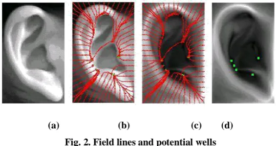
movement is possible. In the Fig. 2, we arranged 62 test pixels around the original image, and these test pixels

form the field lines (the red lines in Fig. 2(b), Fig. 2(c)) and potential wells (the green clusters of test pixels in

Fig. 2(d)). The locations of these wells are extracted by simply noting the coordinates of the clusters of test

pixels that eventually form. These locations are shown in Fig. 2(d), superimposed on force field magnitude. In

order to smooth the field lines, we regulated the number of moving directions as eight. For the horizontal and

vertical moving directions, the increment of each step for test pixels is half of the pixel space distance, while for

the rest directions, half of the diagonal pixels space distance.

(a) (b) (c) (d)

Fig. 2. Field lines and potential wells

However, force exerted on test pixels is a continuity vector, while the locations of test pixels are discrete

magnitude, so it is possible that the locations of potential wells are not in the track of the field lines. Therefore,

this paper marked the locations of each step for a field line and chose the position where the test pixel moved

1295 | P a g e IV. IMPROVED CONVERGENCE FEATURE EXTRACTION

4.1 Adaptive threshold segmentation for convergence images

Hurley found out the threshold for each convergence image by experiment 5, so it needs to adjust the threshold

again and again manually until it could content the visual requirement. Hence it cannot be used directly on large

databases. In this paper, an adaptive threshold segmentation was presented to select the threshold for

convergence images automatically.

Assume there are L-gray levels for an image with N pixels. Let ni be the number of pixels with i gray value. The

threshold t will divide the image into two parts: the foreground and the background. Let the number of pixels in

the background be N1 and that in the foreground be N2. Hence the probability of background is P1= N1/N and

the probability of foreground is P2= N2/N. Let the probability of different gray values in the image be hi= ni/N.

The probability of different gray values in the background and that in the foreground is equation (4) and (5)

respectively.

(4)

(5)

Therefore, the gray center of the background, the gray center of the foreground and that of the whole image are

defined in equation (6), (7) and (8) as m1, m2 and m correspondingly.

(6)

(7)

(8)

Viewing the foreground and the background as two classes, the square of intra-class distance Sb2 ( t) and the

square of inner-class distance Sw2 (t) are defined in the equation (9) and (10) respectively.

(9)

(1

0)

So, the threshold is defined as the max ratio of intra-class and inner-class, defined in the equation (11).

1296 | P a g e Since pixels in the foreground focus on those that of high gray values, the threshold t must be on the right part

of the histogram of each convergence image. We then use the ergodic algorithm to find the threshold for the

converge image.

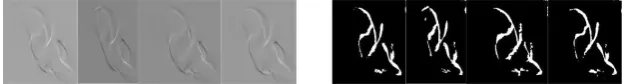
The results of using the adaptive threshold segmentation on one subject of USTB ear database was shown in the

Fig. 3. More detailed description about the USTB ear database could be seen in the Sec. 5.1. Our threshold

segmentation could extract enough foreground pixels from the background pixels, and the threshold

segmentation results are almost close in different samples of the same subject, as shown in the Fig. 3.

Fig. 3. Some results of using the adaptive threshold segmentation

4.2 Classification and recognition

After obtaining the binary image from the convergence image, Hurley used the template matching method for

classification. However, this method is time consuming. In order to speed up the computing process, this paper

adopted a new method which combined the canny operator with the Modified Hausdorff Distance 6 (MHD) to

find the nearest neighbour as the basis for classification.

Unlike most shape comparison methods, the Hausdorff Distance (HD) can be calculated without the explicit

pairing of points in their respective data sets, A and B. This paper adopted the MHD instead of HD simply

because the former is

less sensitive to the noisy points (isolated points) than the latter. Formally, given two finite point sets

A={a1,a2,…,am} and B={b1,b2,…,bn}, the MHD is defined as equation(12). • is some underlying norm over the

point sets A and B. In this paper, we assume that the distance between any two data points is defined as the

Euclidean distance.

V. EXPERIMENTAL RESULTS

5.1 Ear databases-

In this study, two ear databases were tested. The first one is from the Technical University of Madrid of Spain,

just Spain ear database 7 for short. The second one is collected by our research group with various illumination

and pose, named USTB ear database for short. Both ear databases are consisted of 8-bit gray images. There are

17 subjects with 6 different ear samples for each in the Spain ear database and 77 subjects with 4 different ear

samples for each in the USTB ear database. Fig. 4 shows two subjects from different ear databases respectively.

1297 | P a g e Fig. 4. Ear databases. Fig. 4(a) is one subject from the USTB ear database. The leftmost ear image in the Fig.

4(a) was captured from front side with light off, compared to the rightmost one with light on. The second left

ar image has +30 degree deflection from front side, while the third left one has -30 degree deflection from front

side. Figure 4(b) is one subject from the Spain ear database with slight change of illumination and pose.

5.2 Experimental procedure-

In order to improve the speed of calculation, original images were resized to 48 ×30 pixels. After that, the force

field feature extraction and the improved convergence feature extraction could be used.

In the process of force field extraction, we treated the magnitude of force field and the potential wells as two

different kinds of features for ear recognition. The former one was combined with the Principal Component

Analysis (PCA) and Linear Discriminant Analysis (LDA) to reduce the dimension and then the new ear image

was identified by a nearest neighbour classifier. We call this method as F+PCA+LDA for short. The steps of

obtaining potential wells for an original image could refer to the Sec. 3 or Ref. 4.

On the other hand, the ear recognition using improved convergence feature extraction has four steps. Firstly,

using the force field transform to calculate forces of all pixels and after that, translate the original images into

the convergence images; then the adaptive threshold segmentation was used to translate convergence images

into binary images; thirdly, using the canny operator to extract the edge of each binary image and then form the

edge points as a feature vector for this sample; finally, the new ear image was identified by a nearest neighbour

classifier with MHD.

5.3 Experimental results

(1) Potential wells for different samples-

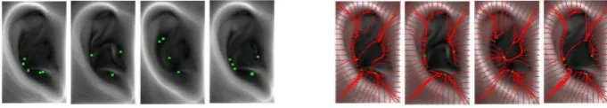
The force field feature extraction based on potential wells was tested on the USTB ear database. However, the

results show that different samples for the same subject possess different numbers and locations of potential

wells. Fig. 5 shows the potential wells for the same subject with four different samples in the USTB ear

database. Applying this method on the other subjects on the USTB ear database, the similar results were

obtained. If there is illumination or pose change among different samples of the same subject, the potential

wells are unstable. It is obvious that the potential wells for the same subject with different samples are various,

so we cannot use the potential wells as the feature to identify different subjects.

Fig. 5. Potential wells for the same subject. In the left four images, green points are potential wells for each ear

sample . In the right four images, red curves are field lines formed by test pixels.

(2) Effectiveness of the adaptive threshold segmentation-

To test the effectivenes of our adaptive threshold segmentation for convergence images, this paper did contrast

1298 | P a g e Table. 1. Results of adaptive threshold segmentation

Ear databases Total of samples Correct numbers Correct rate

USTB 308 300 97.4%

Spain 102 97 95.1%

The standard for right segmentation is that the binary image maintains useful information as much as possible

while not brings in some interference information. Because only in this way can we ensure that the canny

operator could extract the edge effectively and the noisy points would not disturb the calculation of the MHD.

Table 1shows that our method is effective since it almost realizes the automatic selection of threshold for each

convergence image. However, there are still a small number of failed samples. For those failed samples, we

have to choose the threshold by experiment.

(3) Ear recognition based on the force field transform-

In order to test the effect of our improved convergence-based ear recognition algorithm and the F+PCA+LDA

method, we have applied them on two different databases. In the USTB database, we chose the first three ear

samples of every subject as the training samples, and the last image was treated as the testing sample. In the

Spain database, four images for each subject were randomly chosen as the training samples and the remainder

two samples were testing samples. In

addition, classical methods like PCA and LDA for ear recognition were compared with our methods. Table 2

shows the experimental results.

As shown in the Table 2, F+PCA+LDA method has the highest recognition rate 98.7% of all the methods

adopted in this paper. This proves that force field transform could improve the recognition rate. The improved

convergence-based ear recognition method have higher ear recognition rates than the PCA and LDA on the

Spain ear database. When tested on the USTB database, the recognition rates of our methods reduce a little but

still not lower than the LDA and higher than the PCA.

From the data in the Table 2, we concluded that our methods have higher recognition rates than the other two

methods. This is mainly because that our methods are based on the force field transform and the force value of

one pixel with specific location is almost decided by the pixels nearby such location, therefore, they become

less sensitive to the change in the illumination and pose. However, when the change is more obvious, especially

when the gray values of the nearby pixels change a lot, the ear recognition rate will reduce. This explains why

the recognition rates are lower in the USTB database than that in the Spain database when using our two

methods.

Table. 2. Comparison of different ear recognition methods

Methods Spain ear database USTB ear database

PCA 82.4% 92.2%

PCA+LDA 88.2% 93.5%

Improved convergence-based ear recognition 100% 93.5%

1299 | P a g e VI. CONCLUSION

This paper researched three different applications of force field transform for ear recognition. One conclusion

was that the potential wells were not suitable for ear recognition since it is very sensitive to the illumination and

pose change. In the application of convergence field, this paper presented an improved convergence-based ear

recognition algorithm which used the geometrical property of convergence field. It uses the adaptive threshold

segmentation to translate the convergence images into binary images, which has improved the automation of the

algorithm. During the classification process, Modified Hausdorff Distance was adopted to calculate the distance

between different feature vectors extracted by the canny operator, so the computational complexity was

reduced. Furthermore, the algebraic property of force field was also used for ear recognition. Experimental

results prove that ear recognition combined with force field transform is effective, and both the geometrical

property of convergence field and the algebraic property of force field are useful for ear recognition.

REFERENCES

[1] B.Victor, K.Bowyer and S.Sarkar, “An Evaluation of Face and Ear Biometrics,” Proceedings of

InternationalConference on Pattern Recognition, 429-432 (2000).

[2] Mu Zhichun, Yuan Li and Xu Zhengguang, “Shape and Structural Feature Based Ear Recognition,” The 5th

ChineseConference on Biometric Recognition, Guangzhou China, 663-670 (2004).

[3] D.J.Hurley, M.S.Nixon and J.N.Carter, “A New Force Field Transform for Ear and Face Recognition,”

Proceedingof the IEEE International Conference of Image Processing, 25-28(2000).

[4] D.J.Hurley, M.S.Nixon and J.N.Carter, “Force Field Energy Functionals for Image Feature Extraction,”

Image andVision Computing, 20:311-317 (2002).

[5] D.J.Hurley, M.S.Nixon and J.N.Carter, “Force Field Feature Extraction for Ear Biometrics,” Computer

Vision andImage Understanding, 98:491-512 (2005).

[6] D.P.Huttenlocher, G.A.Klanderman and W.J.Rucklidge, “Comparing Images Using the Hausdorff Distance,” IEEETransactions on PAMI, 15(9):850~863 (1993)

[7] M.A.Carreira-Perpinan, Compression Neural Networks for Feature Extraction: Application to Human