PP 2016 16: Arguing about Voting Rules

Arguing about Voting Rules

Olivier Cailloux

Université Paris-Dauphine

PSL Research University CNRS, UMR 7243, LAMSADE

75016 Paris, France

[email protected]

Ulle Endriss

Institute for Logic, Language and Computation University of Amsterdam

P.O. Box 94242

1090 GE Amsterdam, The Netherlands

[email protected]

ABSTRACT

When the members of a group have to make a decision, they can use a voting rule to aggregate their preferences. But which rule to use is a difficult question. Different rules have different properties, and social choice theorists have found arguments for and against most of them. These arguments are aimed at the expert reader, used to mathematical for-malism. We propose a logic-based language to instantiate such arguments in concrete terms in order to help people understand the strengths and weaknesses of different voting rules. Our approach allows us to automatically derive a jus-tification for a given election outcome or to support a group in arguing over which voting rule to use. We exemplify our approach with an in-depth study of the Borda rule.

Keywords

Social Choice Theory; Argumentation; Decision Support

1.

INTRODUCTION

When the members of a committee need to make a deci-sion, they can use avoting rule to aggregate their individ-ual preferences over the available alternatives to arrive at a suitable collective choice. The normative and mathematical analysis of such voting rules is part of social choice the-ory[1], and their algorithmic properties are studied in com-putational social choice[6]. The significant interest amongst AI researchers in social choice theory in recent years, initially sparked by the relevance of the theory to AI applications in areas such as recommender systems, multiagent systems, and search technologies, has opened up several entirely new perspectives on the old problem of voting and has led to novel synergies with a variety of fields in AI and computer science, such as algorithms, knowledge representation, and machine learning. In this paper, we propose to explore a new such synergy and show how to fruitfully apply ideas from automated reasoning and principles of argumentation as studied in AI to a new kind of problem in voting.

There are many different voting rules: Plurality, Veto,

Borda,Copeland,Approval, and so forth [18]. Each of them satisfies certain appealing properties, but none is perfect. Multiple arguments in favour and against different rules

Appears in:Proceedings of the 15th International Conference on Autonomous Agents and Multiagent Systems (AAMAS 2016), J. Thangarajah, K. Tuyls, C. Jonker, S. Marsella (eds.), May 9–13, 2016, Singapore.

Copyright©2016, International Foundation for Autonomous Agents and Multiagent Systems (www.ifaamas.org). All rights reserved.

have been put forward in the literature, starting with the famous dispute between Condorcet and Borda in the 18th century [13]. However, these arguments are dispersed in the specialised literature and are often developed in a highly formal and abstract manner. It therefore is difficult, if not impossible, for an untrained individual to understand them. This means that the members of our committee can hardly have an informed discussion about which voting rule to use. We would like to enable such discussions, by making argu-ments regarding voting rules understandable to non-experts and by providing tools for generating and applying those arguments in concrete situations.

In this paper, we make two contributions towards this long-term goal of enabling informed argumentation about voting rules between non-expert users. First, we develop a general framework for modelling arguments for and against specific outcomes of a voting rule, given a concrete elec-tion instance. This framework allows us to represent many important arguments, either new or taken from the litera-ture, and either highly specific or in the general and abstract form ofaxiomsencoding high-level properties. Because the framework instantiates these arguments on concrete exam-ples, it does not require the audience to understand the ax-ioms in their full generality. Nevertheless, an argument in our framework can still be general in the sense of being ap-plicable to any concrete election instance. Importantly, our framework is not tailored to defend a specific rule: it per-mits the use of arguments in favour of different voting rules. As a second contribution, we instantiate our framework by providing an algorithm for generating arguments justifying the outcome recommended by theBorda rulefor any given election. The technique we use builds on the axiomatisation of that rule developed by Young [21].

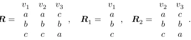
𝑹 =

𝑣1 𝑣2 𝑣3

𝑎 𝑎 𝑐

𝑏 𝑏 𝑏

𝑐 𝑐 𝑎

, 𝑹1= 𝑣1

𝑎 𝑏 𝑐

, 𝑹2= 𝑣2 𝑣3

𝑎 𝑐

𝑏 𝑏

𝑐 𝑎

[image:2.612.56.253.54.96.2]

.

Figure 1: The profiles used in the introductory ex-ample. Each column represents the preference or-dering of one voter.

easy-to-understand sequence of arguments for justifying, for instance, that alternative𝑎is the deserving winner. Such a system might initiate the following dialogue.

System: Consider election𝑹1, involving only voter𝑣1(see also Figure 1). Do you agree that 𝑎, enjoying unanimous support, should win this election?

User: Yes, of course.

System: Now consider election 𝑹2, involving only voters 𝑣₂ and𝑣₃. Do you agree that, for symmetry rea-sons, the outcome should be a three-way tie?

User: Yes, that sounds reasonable.

System: Observe that when we combine 𝑹₁ and 𝑹₂, we obtain our election of interest, namely 𝑹. Do you agree that in this combined election, as there was a three-way tie in𝑹₂,𝑹₁ should be used to decide the winner?

User: Yes, I do.

System: To summarise, you agree that𝑎should win for𝑹.

The reader familiar with the axiomatic method in social choice theory may recognise some of the standard axioms satisfied by the Borda rule at the core of two of these argu-ments (namely Pareto dominance and reinforcement). We will formally introduce these axioms in Section 2. If the user disagrees with one of the steps, the system might try another strategy of arguing in favour of𝑎. Alternatively, we might also ask our system to generate a sequence of arguments to

justify that𝑏should win. △

In this paper, we do not address the rendering of such ar-guments in natural language. Rather, we address the chal-lenge of automatically generating the arguments themselves, expressed in a simple logic-based language. Our framework offers a general solution to the problem of representing such arguments to justify any given outcome for any given elec-tion. Of course, a given user will only find some of the arguments that can be represented in principle convincing in practice. For any “natural” voting rule, one should expect that there will be (by virtue of its naturalness) a convincing set of arguments that can be used to justify the outcomes recommend by that rule. The challenge then is to automat-ically generate a concrete sequence of such arguments for a given outcome to be justified. We provide a solution to this algorithmic problem for the case of the Borda rule.

The remainder of this paper is organised as follows. Sec-tion 2 introduces a logic for specifying reasonableness cri-teria (i.e., axioms) for voting rules. We prove the logic to be complete and demonstrate how it can be used to justify an election outcome. In Section 3 we provide an algorithm for justifying outcomes returned by the Borda rule for ar-bitrary elections. While our main technical contributions concern the challenge of justifying a given election outcome, in Section 4 we briefly explore other further applications of

our approach to richer forms of argumentation about voting rules. Section 5 concludes with a discussion of related work.

2.

GENERAL FRAMEWORK

In this section we introduce a formal model of voting rules for variable electorates, we show how to describe such rules and their properties in a simple logical language, and we then use this language to develop a framework for reasoning and arguing about voting rules.

2.1

Voting Rules

We begin by introducing what is essentially the standard formal model of voting familiar from social choice theory [9, 18], with varying sets of voters.

Let 𝒜, with 𝑚 = |𝒜|, be the finite set of alternatives. Let 𝒫∅(𝒜) denote the powerset of𝒜, excluding the empty set. We use the letters𝐴 ⊆ 𝒜and𝛼 ⊆ 𝒫_∅(𝒜)to designate subsets of alternatives and sets of subsets of alternatives, respectively. We modelpreferencesas (strict) linear orders (transitive, irreflexive, and connected binary relations) over 𝒜. Let𝒩 be the infinite universe of potential voters. A

profile𝑹is a mapping from a finite subset of voters𝑁𝑹⊆ 𝒩 to linear orders over𝒜. For technical reasons, we allow𝑁_𝑹 to be empty, in which case we call𝑹thenull profile. Let𝓡 denote the set of all non-null profiles. Avoting rule𝑓maps each non-null profile𝑹to a non-empty subset of𝒜, the set of (tied) election winners for the profile in question.

Given a profile𝑹, let 𝑹 be the profile consisting of the reverses of the linear orders found in 𝑹. For two profiles 𝑹₁ and 𝑹₂ defined over disjoint sets of voters, we define their sum 𝑹₁⊕ 𝑹₂ as the profile𝑹₁∪ 𝑹₂. (Note that the union of two functions, considered as sets of input-output pairs, defined over disjoint domains, is itself a well-defined function.) In this paper, we will only use addition of profiles in contexts where the identities of the voters do not mat-ter. Therefore, we also define addition over profiles that are not defined over disjoint sets of voters, the addition then being preceded by an arbitrary renaming of the voters of the second profile. Formally, given two profiles𝑹1, 𝑹2 with 𝑁_𝑹

1 ∩ 𝑁𝑹2 ≠ ∅, define 𝑠 as an arbitrary injection

map-ping every voter 𝑖 ∈ 𝑁_𝑹

2 to a voter 𝑠(𝑖) ∈ 𝒩 ∖ 𝑁𝑹1;

de-fine𝑡(𝑹)as the profile{ (𝑠(𝑖), 𝑃 ) ∣ (𝑖, 𝑃 ) ∈ 𝑹 }; and define 𝑹₁⊕ 𝑹₂= 𝑹₁∪ 𝑡(𝑹₂). E.g., for𝑹 = { (𝑖, (𝑎, 𝑏)) },𝑹 ⊕ 𝑹is { (𝑖, (𝑎, 𝑏)), (𝑖′_{, (𝑎, 𝑏)) }, with𝑖}′_{≠ 𝑖an arbitrary voter. A} pro-file𝑹may be multiplied by a natural number𝑘 ∈ ℕ, defined in the natural way as repeated addition with copies of itself and denoted by𝑘𝑹. Multiplying a profile by zero yields the null profile. Throughout this paper, natural numbers are taken to include zero.

2.2

Logical Language and Axioms

To formally describe voting rules we will make use of the language of propositional logic over the set of atomic propo-sitions{ 𝑝_𝑹,𝐴 ∣ 𝑹 ∈ 𝓡, ∅ ⊂ 𝐴 ⊆ 𝒜 }. This set includes one atom for every possible non-null profile𝑹 and every possi-ble non-empty subset𝐴of alternatives. The languageℒ is the set of all formulæ that can be formed using these atoms and the propositional connectives¬, ∧, ∨, and→as well as the special propositions⊤and⊥, in the usual manner [19]. Aliteralis an atom or its negation; aclauseis a disjunction of literals.

𝑝𝑹,𝐴if𝑓(𝑹) = 𝐴and the valueF(false) otherwise. That is, 𝑝𝑹,𝐴 is true if𝑓 chooses𝐴 as the set of winners whenever the voters vote as in profile𝑹. The definition of𝑣_𝑓 extends to the whole set of formulæ using the usual semantics of propositional logic. We say that𝑣𝑓 satisfiesa set of formulæ

iff it assigns the valueTto every formula in the set. To make the semantics of the atoms explicit in the lan-guage, we from now on write[𝑹 ↦ 𝐴]instead of𝑝𝑹,𝐴. We also write [𝑹 ∈⟼ 𝛼], for any non-empty 𝛼 ⊆ 𝒫∅(𝒜), as a shorthand for⋁

𝐴∈𝛼[𝑹 ↦ 𝐴]. We will refer to such clauses involving only one profile, i.e., formulæ specifying the possi-ble sets of winners for a given profile, asuni-profile clauses. We can express familiar as well as new axioms of social choice theory in our language. We call any such rendering of an axiom inℒanℒ-axiom. Formally, anℒ-axiom is simply a set of formulæ. Here are some examples forℒ-axioms.

Dom Dominancepostulates that a Pareto-dominated native (i.e., an alternative to which some other alter-native is preferred by every voter) should not win. The formulæ are, for each 𝑹 ∈ 𝓡, [𝑹 ∈⟼ 𝒫∅(𝑈𝑹)], where𝑈𝑹is the set of alternatives that are not Pareto-dominated in𝑹.

Anon Anonymity asks for symmetry w.r.t. voters: for all 𝑹 ∈ 𝓡, ∅ ⊂ 𝐴 ⊆ 𝒜,𝑁′_{⊆ 𝒩, bijections𝜎 ∶ 𝑁}′_{→ 𝑁}

𝑹, anonymity requires[𝑹 ↦ 𝐴] → [(𝑹 ∘ 𝜎) ↦ 𝐴].

Cond This axiom says that, if there is aCondorcet winner

(an alternative beating all other alternatives in one-on-one majority contests), then it should be the sole winner: thus, for each profile 𝑹with Condorcet win-ner𝑎, it requires[𝑹 ↦ { 𝑎 }].

Reinf Reinforcement requires that, when joining two pro-files for which the winning sets have a non-empty inter-section, the resulting profile must have that intersec-tion as the only winners: for each𝑹₁, 𝑹₂, 𝑁_𝑹

1∩𝑁𝑹2=

∅, 𝐴1 ∩ 𝐴2 ≠ ∅, reinforcement imposes the formula ([𝑹1↦ 𝐴1] ∧ [𝑹2↦ 𝐴2]) → [𝑹1⊕ 𝑹2↦ 𝐴1∩ 𝐴2].

SymCanc Symmetric cancellationsays that, when a profile consists of a linear order and its inverse, then the only reasonable outcome is the full set of alternatives: for each such profile𝑹, this axiom thus requires[𝑹 ↦ 𝒜].

Reinforcement, also known as consistency in the litera-ture, was introduced by Young [21]. Like dominance and the Condorcet principle, it is one of the classical axioms considered in social choice theory [9]. SymCancis anad hoc, but intuitively appealing, axiom we will use in Example 2.

An ℒ-axiom may also be limited to capturing what an adequate behaviour is on a few specific cases, or even just a single specific case. As an example, let us inspect the argument put forward by Fishburn [8, p. 544] against the Condorcet principle. Consider the profile𝑹_𝐹 shown in Fig-ure 2, involving9alternatives and101voters.1 _{Observe that}

𝑤is the Condorcet winner, as it is preferred to any other alternative by 51 out of 101 voters. Yet, it is intuitively appealing to postulate that alternative𝑎 is in fact a more deserving winner of this election. This may be seen by look-ing at the numbers of times alternatives𝑎 and 𝑤obtain a given rank (also displayed in Figure 2).

1_{Fishburn explains his argument without giving a fully}

worked out example. The profile used here is taken from http://rangevoting.org/FishburnAntiC.html.

number of voters

31 19 10 10 10 21 𝑤 𝑎

1 𝑎 𝑎 𝑓 𝑔 ℎ ℎ 1 0 50

2 𝑏 𝑏 𝑤 𝑤 𝑤 𝑔 2 30 0

3 𝑐 𝑐 𝑎 𝑎 𝑎 𝑓 3 0 30

4 𝑑 𝑑 ℎ ℎ 𝑓 𝑤 4 21 0

5 𝑒 𝑒 𝑔 𝑓 𝑔 𝑎 5 0 21

6 𝑤 𝑓 𝑒 𝑒 𝑒 𝑒 6 31 0

7 𝑔 𝑔 𝑑 𝑑 𝑑 𝑑 7 0 0

8 ℎ ℎ 𝑐 𝑐 𝑐 𝑐 8 0 0

9 𝑓 𝑤 𝑏 𝑏 𝑏 𝑏 9 19 0

Figure 2: The profile Fishburn uses to argue against the Condorcet property; and the number of voters placing alternative 𝑤or𝑎at a given rank.

FvsC TheFishburn-versus-Condorcetℒ-axiomis defined as the formula[𝑹_𝐹↦ { 𝑎 }].

2.3

Reasoning about Voting Rules

Now that we have a logical language for describing the outcomes of a voting rule for different profiles in place, we want to be able to reason about statements in this language. To this end, we first fix some additional terminology regard-ing the relationship betweenℒ-axioms and voting rules.

Definition 1. An ℒ-axiomatisation is a set of ℒ-axioms. A voting rule 𝑓 conforms to theℒ-axiomatisation 𝐽 iff 𝑣𝑓 satisfies allℒ-axioms𝑗in𝐽. Anℒ-axiomatisation𝐽 is con-sistent iff some voting rule conforms to it. 𝐽 characterises 𝑓 iff𝑓 is the only voting rule conforming to it.

Given a set of assumptions of what makes a good voting rule, expressed in the form of anℒ-axiomatisation, we want to be able to decide whether a given claim about a given set of alternatives being the deserving winners for a given profile logically follows from those assumptions. In other words, we want to be able to justify election outcomes in terms of a givenℒ-axiomatisation. The next definition fixes the semantics of what it means for such a claim to be valid.

Definition 2. Consider anℒ-axiomatisation 𝐽 and a for-mula𝜑in our language. We say that𝜑is avalid claimgiven 𝐽 iff𝑣_𝑓(𝜑) =Tfor all voting rules𝑓 conforming to𝐽.

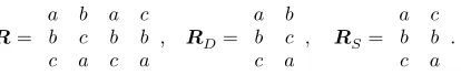
𝑹 =

𝑎 𝑏 𝑎 𝑐

𝑏 𝑐 𝑏 𝑏

𝑐 𝑎 𝑐 𝑎

, 𝑹𝐷= 𝑎 𝑏 𝑏 𝑐 𝑐 𝑎

, 𝑹𝑆= 𝑎 𝑐 𝑏 𝑏 𝑐 𝑎 .

Figure 3: The profiles used in Example 2. Each col-umn represents the preference ordering of one voter.

in𝐽 as a demonstration that𝜑can be inferred from𝐽 and 𝜅, i.e., that (⋃ 𝐽 ) ∪ 𝜅 ⊢ 𝜑. Natural deduction [19], which is widely regarded as producing proofs of good readability, is particularly suited to this purpose, but any other system that is sound and complete for propositional logic could be used as well.

Definition 3. Aproof of claim 𝜑grounded inℒ -axioma-tisation𝐽 is a natural deduction proof for(⋃ 𝐽 ) ∪ 𝜅 ⊢ 𝜑.

For the purposes of presenting examples, in this paper, we will take certain shortcuts and omit the detailed derivation of simple facts about propositional logic. We will justify such steps as being inferred ‘by propositional reasoning’ (PR), together with a reference to the premises used. What is important in view of our ultimate goal of justifying election outcomes to users is that any such propositional reasoning step can be decomposed into a sequence of basic steps in a natural deduction proof, which can then be translated into an argument in natural language that can be explained to a non-expert user [2, 14, 20].

[image:4.612.57.264.52.86.2]

Example 2. We prove below, on the basis of ℒ-axioms Dom,SymCanc, andReinfdefined earlier, that the profile𝑹 of Figure 3 must have as winners either{ 𝑎 },{ 𝑏 }, or{ 𝑎, 𝑏 }, i.e., that𝑐should not win. Each line consists of a formula we have shown to be true, followed by the justification for that proof step. The profiles𝑹𝐷and𝑹𝑆are also defined in Figure 3. Note that𝑹 = 𝑹_𝐷⊕ 𝑹_𝑆.

1. [𝑹𝐷⟼ { { 𝑎 } , { 𝑏 } , { 𝑎, 𝑏 } }] (∈ Dom) 2. [𝑹_𝑆↦ { 𝑎, 𝑏, 𝑐 }] (SymCanc)

3. ([𝑹𝐷↦ { 𝑎 }] ∧ [𝑹𝑆↦ { 𝑎, 𝑏, 𝑐 }]) → [𝑹 ↦ { 𝑎 }] (Reinf) 4. ([𝑹𝐷↦ { 𝑏 }] ∧ [𝑹𝑆↦ { 𝑎, 𝑏, 𝑐 }]) → [𝑹 ↦ { 𝑏 }] (Reinf) 5. ([𝑹𝐷↦ { 𝑎, 𝑏 }] ∧ [𝑹𝑆↦ { 𝑎, 𝑏, 𝑐 }]) → [𝑹 ↦ { 𝑎, 𝑏 }] (Reinf) 6. [𝑹_𝐷↦ { 𝑎 }] → [𝑹 ↦ { 𝑎 }] (PR from 2 & 3)

7. [𝑹_𝐷↦ { 𝑏 }] → [𝑹 ↦ { 𝑏 }] (PR from 2 & 4) 8. [𝑹𝐷↦ { 𝑎, 𝑏 }] → [𝑹 ↦ { 𝑎, 𝑏 }] (PR from 2 & 5) 9. [𝑹𝐷↦ { 𝑎 }] ∨ [𝑹𝐷↦ { 𝑏 }] ∨ [𝑹𝐷↦ { 𝑎, 𝑏 }] (rewrite 1) 10. [𝑹 ↦ { 𝑎 }] ∨ [𝑹 ↦ { 𝑏 }] ∨ [𝑹 ↦ { 𝑎, 𝑏 }] (PR from 6–9) 11. [𝑹 ∈⟼ { { 𝑎 } , { 𝑏 } , { 𝑎, 𝑏 } }] (rewrite 10)

Each of these steps is simple enough to be rendered in natural language, so as to be presented to a non-expert user, just as in Example 1. For instance, steps 2 and 3 directly correspond to steps also present in Example 1, while step 6 might be explained by pointing out that when two premises imply a conclusion, then that conclusion is implied by the first premise alone once we have established that the second

premise is in fact true. △

Remark 1. It is important to understand that twoℒ -ax-ioms may be equivalent, logically speaking, while leading to proofs that differ in terms of how easy or difficult they are to understand for a human reader. In our proposal, it is im-portant to chooseℒ-axioms not only according to what they

entail (their logical power), but also according to the ease of understanding them. This is similar to the general goal of axiomatising a function: we search for axioms that have, as much as possible, an intuitive content. In our case, how-ever, anℒ-axiomatisation is good if it strikes an appropriate balance between the lengths of proofs it produces and the intuitiveness of the concrete instantiations of theℒ-axioms it contains. As an illustration, Reinf could be changed in order to shorten the proof of Example 2. A modifiedReinf would say, for example, that a profile associated with a set of possible sets of winners, when added to a profile that has the full set𝒜as the winners, must still be associated with the same set of possible sets of winners. This axiom would yield, in a single step, that[𝑹𝐷⟼ { { 𝑎 } , { 𝑏 } , { 𝑎, 𝑏 } }] ∧ [𝑹∈ 𝑆↦ { 𝑎, 𝑏, 𝑐 }]) → [𝑹 ∈⟼ { { 𝑎 } , { 𝑏 } , { 𝑎, 𝑏 } }].

We now want to show that, with our definition of proofs, we can prove only and all claims that indeed are valid.

Theorem 1 (Completeness). For anyℒ -axiomatisa-tion𝐽 and any claim𝜑, there exists a proof of𝜑grounded in𝐽 iff𝜑is valid given𝐽.

Proof. The theorem follows from the (soundness and) completeness of natural deduction for classical propositional logic [19], together with the fact that there exists a bijection between voting rules conforming to𝐽 and models satisfying 𝐽and𝜅. Indeed, for each𝑓conforming to𝐽, the correspond-ing model𝑣_𝑓 satisfies𝐽 and𝜅. Now take any𝑣satisfying𝐽 and𝜅. As the model satisfies𝜅, we can define a rule𝑓from that model, taking𝑓(𝑹) = 𝐴when the model says[𝑹 ↦ 𝐴] is true. Because𝑣 = 𝑣_𝑓,𝑓conforms to𝐽.

Thus, while our logical language permits us to speak about voting rules by making arbitrary claims about the possible sets of winners for a given profile, we now have a proof sys-tem in place for deriving any valid such claim from a given axiomatisation provided in the same language. The render-ings of the axioms themselves may be long and unwieldy (e.g., Dom explicitly lists all undominated alternatives for every profile), but the concrete proofs produced nevertheless can be expected to be relatively simple and human-readable (as seen in Example 2). Finding the right concrete profiles (e.g., 𝑹𝐷 and 𝑹𝑆 in Example 2) to use in a proof may be hard, but reading an existing proof is easy. In Section 3 we will address this challenge of actually producing proofs.

3.

JUSTIFYING BORDA OUTCOMES

TheBorda ruleis one of the most important voting rules in the literature [18]. Under this rule, an alternative𝑎earns as many points from a given voter as that voter ranks other alternatives below 𝑎. The Borda score of an alternative is the sum of points it earns in this manner; the alternatives with the highest Borda score win. For our purposes, it will be convenient to use the following alternative definition.

Definition 4. Given a profile, the beta score of an alter-native is the sum of the numbers of alteralter-natives it beats in each linear order, minus the sum of the numbers of alterna-tives it is beaten by in each linear order. Under theBorda rule𝑓_𝐵the alternatives with the highest beta score win.

recall that𝑚is the number of alternatives. The beta score, for a given voter, is𝑏 − (𝑚 − 1 − 𝑏) = 2𝑏 − (𝑚 − 1), where𝑏 is the Borda score of that same voter. Thus, the total beta score of an alternative is twice its total Borda score minus 𝑛(𝑚 − 1).

In this section we want to use our logic to justify a given outcome of Borda. That is, starting from any profile 𝑹∗_, we want to be able to give a proof, grounded inℒ-axioms that are as appealing as possible, for the claim that the only “reasonable” winners must be the ones Borda picks (pro-vided the reader of the argument finds these instantiations of axioms indeed reasonable). We will thus, first, present anℒ-axiomatisation of Borda and, second, provide an algo-rithm that, given any𝑹∗_{, builds a proof for[𝑹}∗_{↦ 𝑓}

𝐵(𝑹∗)].

3.1

Borda

ℒ

-Axiomatisation

To present theℒ-axiomatisation that we will use to argue in favour of Borda, we require a few definitions. Fix an arbitrary linear order≻on𝒜. (We will use the alphabetic ordering in our illustrative examples.)

Definition 5. Theelementary profile𝑹𝐴

𝑒,∅ ⊂ 𝐴 ⊆ 𝒜, has two voters and is defined as follows. Let 𝑘 = ≻|_𝐴 be the restriction of≻on𝐴and letℓ = ≻|_𝒜∖𝐴. The first voter has the linear order defined by𝑘thenℓ; the second has𝑘thenℓ.

Example 3. The elementary profile𝑹𝑒{ 𝑎,𝑏 }corresponding to 𝐴 = { 𝑎, 𝑏 }, with 𝒜 = { 𝑎, 𝑏, 𝑐, 𝑑 }, is composed of the linear orders(𝑎, 𝑏, 𝑐, 𝑑)and(𝑏, 𝑎, 𝑑, 𝑐). △

Let us call a bijection 𝑆 on 𝒜 an 𝑚-cycle if (𝒜, 𝑆) is a strongly connected graph, thus, if 𝑆 represents a cycle that visits each alternative in𝒜exactly once. It is formally defined as a set of pairs of alternatives, but we will denote such a cycle using a tuple of alternatives, where the first and last alternatives are equal, and all other alternatives appear exactly once. For example,⟨𝑎, 𝑐, 𝑏, 𝑑, 𝑎⟩denotes the 𝑚-cycle{ (𝑎, 𝑐), (𝑐, 𝑏), (𝑏, 𝑑), (𝑑, 𝑎) }in{ 𝑎, 𝑏, 𝑐, 𝑑 }. This cycle can also be represented as⟨𝑏, 𝑑, 𝑎, 𝑐, 𝑏⟩. We say that a cycle in𝒜generates𝑚 = |𝒜| linear orders on𝒜, in the natural way. For example,⟨𝑎, 𝑐, 𝑏, 𝑎⟩generates(𝑎, 𝑐, 𝑏),(𝑐, 𝑏, 𝑎), and (𝑏, 𝑎, 𝑐). We write linear orders with regular parentheses(⋯) to distinguish them from cycles ⟨⋯⟩. Conversely, observe that a linear order involving all alternatives in𝒜is generated by exactly one𝑚-cycle.

Definition 6. Thecyclic profile𝑹𝑆

𝑐, with𝑆an𝑚-cycle, is the profile composed of all𝑚linear orders generated by𝑆.

Example 4. The cyclic profile𝑹𝑐⟨𝑎,𝑏,𝑐,𝑑,𝑎⟩corresponding to 𝑆 = ⟨𝑎, 𝑏, 𝑐, 𝑑, 𝑎⟩ with 𝒜 = { 𝑎, 𝑏, 𝑐, 𝑑 } has the preference orders(𝑎, 𝑏, 𝑐, 𝑑),(𝑏, 𝑐, 𝑑, 𝑎),(𝑐, 𝑑, 𝑎, 𝑏)and(𝑑, 𝑎, 𝑏, 𝑐). △

Adelta vector𝛿is a mapping from≻to the rationals: such a vector has(𝑚

2)coordinates, each mapping a pair of alter-natives to a rational number. For every pair of alteralter-natives (𝑎, 𝑏) ∈ ≻, define 𝛿_𝑏𝑎 = −𝛿_𝑎𝑏 (slightly abusing notation). The set of delta vectors, denoted by 𝛿 , together with addi-tion and multiplicaaddi-tion by a raaddi-tional defined in the natural way, is a vector space.

Definition 7. For any profile𝑹, thedelta vector𝛿𝑹_maps every(𝑎, 𝑏) ∈ ≻to the signed number of victories of𝑎against 𝑏, i.e.,𝛿𝑹

𝑎𝑏is the number of voters who prefer 𝑎to𝑏 minus the number of voters who prefer𝑏to𝑎.

Thus,𝛿𝑹_{represents theweighted majority graphof𝑹.} We say that two profiles𝑹and𝑹′_{cancelwhen𝛿}𝑹_{= 𝛿}𝑹′

, thus when𝑹and𝑹′_{have the same weighted majority graph,} or equivalently, observing that𝛿𝑹_{= −𝛿}𝑹_{, when𝛿}𝑹⊕𝑹′

= 𝟎, where𝟎is the zero vector.

Below is theℒ-axiomatisation that we use for the Borda rule. The fact that it is acorrectaxiomatisation of the Borda rule will follow from Theorem 2 below. As discussed below, in Section 3.4, our axiomatisation is very similar but not identical to the axiomatisation given by Young [21].

Elem For any elementary profile𝑹𝐴

𝑒, the only reasonable set of winners is𝐴: for all∅ ⊂ 𝐴 ⊆ 𝒜,[𝑹𝐴

𝑒 ↦ 𝐴].

Cycl For any cyclic profile𝑹𝑆

𝑐, the only reasonable set of winners is𝒜: for all𝑚-cycles𝑆,[𝑹𝑆

𝑐↦ 𝒜].

Canc If all pairs of alternatives(𝑎, 𝑏)are such that𝑎is pre-ferred to𝑏as many times as𝑏is to𝑎, then the set of winners must be𝒜: for all𝑹such that𝛿𝑹

𝑎𝑏= 0for all (𝑎, 𝑏) ∈ ≻,[𝑹 ↦ 𝒜].

Reinf Reinforcement, as defined earlier (cf. Section 2.2).

Reinf-sub Subtracting a profile with a full winner-set does not change the outcome. For all 𝑹, 𝑹′_{, ∅ ⊂ 𝐴 ⊆ 𝒜:} ([𝑹 ⊕ 𝑹′_{↦ 𝐴] ∧ [𝑹}′_{↦ 𝒜]) → [𝑹 ↦ 𝐴].}

Simp If a profile consists of a repetition of the same sub-profile, then the sub-profile must have the same win-ners (i.e., we can simplify): for all 𝑹, 2 ≤ 𝑘 ∈ ℕ, ∅ ⊂ 𝐴 ⊆ 𝒜,[𝑘𝑹 ↦ 𝐴] → [𝑹 ↦ 𝐴].

We denote ourℒ-axiomatisation by𝐽𝐵, the set of all six sets of formulæ just defined.

Remark 3. Observe thatSimpandReinf-sublogically fol-low from Reinf, i.e., they are in fact not required for the characterisation itself. We introduce them nevertheless, as explained in Remark 1, because they can shorten proofs, and because we assume they will appear sufficiently intuitive to the reader of such proofs to be used without requiring sep-arate justification themselves.

3.2

An Example

Consider the set of alternatives 𝒜 = { 𝑎, 𝑏, 𝑐, 𝑑 } and a profile𝑹∗_{composed of the two preference orders (𝑎, 𝑏, 𝑑, 𝑐)} and(𝑐, 𝑏, 𝑎, 𝑑). Observe that Borda selects{ 𝑎, 𝑏 }as winners for this profile. We will now build a proof grounded in 𝐽_𝐵 of the claim[𝑹∗_{↦ { 𝑎, 𝑏 }].}

The proof consists of two parts. First (steps 1–8 in this example), we define a profile 𝑹′ _{that is the sum of several} profiles for which the winners are uncontroversial, either be-cause ofElemor because ofCycl, and use this to argue that our Borda winners should win for𝑹′_{. For our example, let} 𝑹𝐸= 𝑹

{ 𝑎,𝑏 }

𝑒 ⊕ 2𝑹𝑒{ 𝑎,𝑏,𝑐 },𝑹𝐶= 𝑹 ⟨𝑎,𝑑,𝑐,𝑏,𝑎⟩

𝑐 ⊕ 𝑹𝑐⟨𝑎,𝑏,𝑑,𝑐,𝑎⟩, and 𝑹′_{= 𝑹}

1. [𝑹𝑒{ 𝑎,𝑏 }↦ { 𝑎, 𝑏 }](Elem) 2. [𝑹𝑒{ 𝑎,𝑏,𝑐 }↦ { 𝑎, 𝑏, 𝑐 }](Elem) 3. [𝑹𝑐⟨𝑎,𝑑,𝑐,𝑏,𝑎⟩↦ 𝒜](Cycl) 4. [𝑹𝑐⟨𝑎,𝑏,𝑑,𝑐,𝑎⟩↦ 𝒜](Cycl)

5. ((1) ∧ (2)) → [𝑹𝐸↦ { 𝑎, 𝑏 }](Reinf) 6. ((3) ∧ (4)) → [𝑹_𝐶↦ 𝒜](Reinf)

7. ([𝑹_𝐸↦ { 𝑎, 𝑏 }] ∧ [𝑹_𝐶↦ 𝒜]) → [𝑹′_{↦ { 𝑎, 𝑏 }](Reinf)} 8. [𝑹′_{↦ { 𝑎, 𝑏 }](PR from 5–7)}

9. [4𝑹∗_{⊕ 4𝑹}∗_{↦ 𝒜](Canc)}

10. ([4𝑹∗_{⊕ 4𝑹}∗_{↦ 𝒜] ∧ [𝑹}′_{↦ { 𝑎, 𝑏 }]) → [4𝑹}∗_{⊕ 4𝑹}∗_{⊕ 𝑹}′_↦ { 𝑎, 𝑏 }](Reinf)

11. [4𝑹∗_{⊕ 4𝑹}∗_{⊕ 𝑹}′_{↦ { 𝑎, 𝑏 }](PR from 8–10)}

12. [4𝑹∗_{⊕ 𝑹}′_{↦ 𝒜](Canc)}

13. ([4𝑹∗_{⊕ 4𝑹}∗_{⊕ 𝑹}′_{↦ { 𝑎, 𝑏 }] ∧ [4𝑹}∗_{⊕ 𝑹}′_{↦ 𝒜]) → [4𝑹}∗_↦ { 𝑎, 𝑏 }](Reinf-sub)

14. [4𝑹∗_{↦ { 𝑎, 𝑏 }](PR from 11–13)} 15. [4𝑹∗_{↦ { 𝑎, 𝑏 }] → [𝑹}∗_{↦ { 𝑎, 𝑏 }](Simp)} 16. [𝑹∗_{↦ { 𝑎, 𝑏 }](PR from 14 & 15)}

Simplifications are possible. For instance, step 8 could be presented to a user as following directly from steps 1–4, together withReinfand basic propositional reasoning.

3.3

The General Algorithm

We now define an algorithm,Borda-expl, which, given any profile𝑹∗_{, builds a proof grounded in𝐽}

𝐵of the claim[𝑹∗↦ 𝑓_𝐵(𝑹∗_{)], i.e., a justification for the Borda outcome. Our} proofs all have the same structure as in the example above; only the concrete profiles used along the way differ. We show how to compute a natural number 𝑟, a profile 𝑹_𝐸 that is the sum of several elementary profiles, and a profile 𝑹𝐶 that is the sum of several cyclic profiles such that, for 𝑹′ _{= 𝑟𝑹}

𝐸⊕ 𝑹𝐶, (𝑖) the winners for𝑹′ are 𝑓𝐵(𝑹∗), and (𝑖𝑖) 𝑟𝑚𝑹∗_and𝑹′_{have the same weighted majority graph.}

First, let us define 𝑹𝐸. Define a beta vector as a vector mapping alternatives from𝒜to rationals, with the condi-tion that it sums to zero. The set of beta vectors, denoted by 𝛽, together with addition and multiplication by a ra-tional defined in the natural way, is a vector space. We write 𝛽𝑹 _{= ⟨𝛽}𝑹

𝑎, 𝑎 ∈ 𝒜⟩ for the beta vector correspond-ing to a profile 𝑹, where 𝛽𝑹

𝑎 denotes the beta score of 𝑎 in𝑹. Name alternatives𝑎1, 𝑎2, … , 𝑎𝑚 by decreasing beta score in 𝑹∗_{, thus 𝛽}𝑹∗

𝑎1 ≥ 𝛽

𝑹∗

𝑎2 ≥ … ≥ 𝛽

𝑹∗

𝑎𝑚. Define 𝑹𝐸 =

⨁𝑚−1 𝑖=1

𝛽𝑹∗ 𝑎𝑖−𝛽𝑹∗𝑎𝑖+1

2 𝑹

{ 𝑎1,…,𝑎𝑖}

𝑒 .

Remark 4. This definition of 𝑹𝐸 is legal as the coeffi-cients are natural numbers: (𝛽𝑹∗

𝑎𝑖 − 𝛽

𝑹∗

𝑎𝑖+1) is even because,

depending on𝑚, either all beta scores are even, or all are odd (as may be seen by revisiting Remark 2).

We can now show that𝑹𝐸 has the same beta scores as 𝑚𝑹∗_{, which is equivalent to a result due to Young [21].}

Lemma 1 (Young, 1974). With the above definitions, for each𝑎 ∈ 𝒜: 𝛽𝑹𝐸

𝑎 = 𝛽𝑚𝑹

∗

𝑎 .

Proof. First observe that ∀∅ ⊂ 𝐴 ⊆ 𝒜, 𝛽𝑹𝑒𝐴

𝑎 equals 2(𝑚 − |𝐴|) if 𝑎 ∈ 𝐴 and −2|𝐴| if 𝑎 ∉ 𝐴. Write 𝛽_𝑎 instead of 𝛽𝑹∗

𝑎 . Now 𝛽 𝑹_𝐸

𝑎_𝑖 = ∑𝑖−1_𝑗=1

𝛽_𝑎𝑗−𝛽_𝑎𝑗+1

2 (−2𝑗) +

∑𝑚−1 𝑗=𝑖

𝛽_𝑎𝑗−𝛽_𝑎𝑗+1

2 2(𝑚 − 𝑗) = ∑

𝑚−1

𝑗=1 (𝛽𝑎𝑗 − 𝛽𝑎𝑗+1)(−𝑗) +

∑𝑚−1_𝑗=𝑖 (𝛽𝑎_𝑗− 𝛽𝑎_𝑗+1)𝑚 = (∑ 𝑚−1

𝑗=1 −𝛽𝑎𝑗) + (𝑚 − 1)𝛽𝑎𝑚+ 𝑚𝛽𝑎𝑖−

𝑚𝛽_𝑎

𝑚 = (∑

𝑚

𝑗=1−𝛽𝑎𝑗) + 𝑚𝛽𝑎𝑖. The claim now follows from

∑_𝑎∈𝒜𝛽𝑎= 0.

Thus,𝑹_𝐸 and 𝑚𝑹∗_{have the same Borda winners.}2 _We

now have to define𝑹′_{. Recall that we want𝑹}′_{and𝑟𝑚𝑹}∗_to have equal weighted majority graphs for some𝑟. Thus, our objective is to obtain𝛿𝑹′

= 𝛿𝑟𝑚𝑹∗

. Assume we can find a set of𝑚-cycles𝒮and rationals⟨𝑞_𝑆, 𝑆 ∈ 𝒮⟩that solve the linear system of equations 𝛿𝑚𝑹∗

= 𝛿𝑹_{𝐸+ ∑}

𝑆∈𝒮𝑞𝑆𝛿𝑹

𝑆

𝑐. (We will

shortly define𝒮 and prove that this system always admits a solution.) Because𝛿𝑹𝑆

𝑐 = −𝛿𝑹−𝑆𝑐 , where−𝑆 denotes the

inverse cycle of 𝑆, we can then choose coefficients 𝑞_𝑆 that are all non-negative. Then, it remains only to define 𝑟 as the smallest strictly positive integer such that{ 𝑟𝑞𝑆, 𝑆 ∈ 𝒮 } are all natural numbers, and to define 𝑹𝐶 = ⨁_𝑆𝑟𝑞𝑆𝑹𝑆𝑐. Indeed,𝑹′_{= 𝑟𝑹}

𝐸⊕ 𝑹𝐶 then has the same winners as𝑹𝐸 (hence, the same as 𝑹∗_{), and𝛿}𝑟𝑚𝑹∗

= 𝛿𝑹′

. (The comment made in Footnote 2 applies here as well.)

It remains to show that the system above can be solved. Indeed, even considering all(𝑚 − 1)! 𝑚-cycles as the set𝒮, the claim that such a system can always be solved requires a proof. Furthermore, our proof permits to use a quadratic— instead of a factorial—number of unknowns, as we define precisely which cycles𝒮must contain.

Lemma 2. There exists a set of𝑚-cycles𝒮such that, for any two profiles 𝑹∗_{, 𝑹}

𝐸 satisfying 𝛽𝑚𝑹

∗

= 𝛽𝑹𝐸, there exist

rationals𝑞_𝑆 with∑_𝑆∈𝒮𝑞_𝑆𝛿𝑹𝑆

𝑐 = 𝛿𝑚𝑹∗− 𝛿𝑹𝐸.

In order to prove Lemma 2, we will first define a beta trans-formation 𝛽, a linear transformation from̂ 𝛿 to 𝛽. We

will then show that𝛿𝑚𝑹∗

− 𝛿𝑹𝐸 belongs to its kernel𝒦( ̂𝛽)

(Lemma 3). Next, we will define 𝒮 and show that we can find rationals𝑞𝑆with∑_𝑆∈𝒮𝑞𝑆𝛿𝑹

𝑆

𝑐 = 𝛿, for any delta vector

𝛿 ∈ 𝒦( ̂𝛽). Equivalently, defining𝜌 = { 𝛿𝑹𝑆

𝑐, 𝑆 ∈ 𝒮 }, we will

show that𝜌spans𝒦( ̂𝛽)(Lemma 4). In order to do this, ob-serving that𝜌 ⊆ 𝒦( ̂𝛽), we will show thatdim 𝒦( ̂𝛽) = dim 𝜌, or equivalently, that𝜌hasdim 𝒦( ̂𝛽)independent vectors.

Define the beta transformation 𝛽(𝛿)̂ of a delta vector 𝛿 as the following beta vector: 𝛽(𝛿)̂ 𝑎 = ∑_{𝑏∈𝒜∖{ 𝑎 }}𝛿𝑎𝑏. Let

𝒦( ̂𝛽)denote the kernel of the beta transformation, the vec-tor space of vecvec-tors𝛿 such that𝛽(𝛿) = 𝟎̂ . Because 𝛽̂is a surjective linear transformation from 𝛿 of dimension(𝑚

2)to 𝛽 of dimension𝑚 − 1,dim 𝒦( ̂𝛽) = (𝑚

2) − (𝑚 − 1).

Lemma 3 (Young, 1974). For any two profiles𝑹∗_{, 𝑹} 𝐸

satisfying 𝛽𝑚𝑹∗

= 𝛽𝑹_𝐸,𝛿𝑚𝑹∗

− 𝛿𝑹_{𝐸∈ 𝒦( ̂𝛽).}

Proof. Because𝛽̂is linear and for any𝑹,𝛽𝑹_=𝛽(𝛿̂ 𝑹_), we get𝛽(𝛿̂ 𝑚𝑹∗

− 𝛿𝑹_{𝐸) = 𝛽}𝑚𝑹∗

− 𝛽𝑹_{𝐸. By the hypothesis of} this lemma, this equals zero. Thus,𝛿𝑚𝑹∗

− 𝛿𝑹_{𝐸∈ 𝒦( ̂𝛽).}

2_If𝑹

𝑆𝑎𝑏 _𝑆𝑎𝑐 _𝑆𝑏𝑐

〈𝑎, 〈𝑏, 〈𝑏,

𝑏, 𝑎, 𝑐,

𝑐, 𝑐, 𝑎,

𝑑, 𝑑, 𝑑,

𝑎〉 𝑏〉 𝑏〉

𝒮

𝑀 𝛿𝑹𝑆𝑎𝑏

𝑐 𝛿𝑹𝑆𝑎𝑐𝑐 𝛿𝑹𝑆𝑏𝑐𝑐

𝑎𝑏 2 −2 0

𝑎𝑐 0 2 −2

𝑎𝑑 −2 0 2

𝑏𝑐 2 0 2

𝑏𝑑 0 −2 −2

𝑐𝑑 2 2 0

𝑇 𝑎𝑏 𝑎𝑐 𝑎𝑑 𝑏𝑐 𝑏𝑑 𝑐𝑑

𝑎𝑏 1 0 −1 0 1 0

𝑎𝑐 0 1 −1 0 0 1

𝑏𝑐 0 0 0 1 −1 1

𝑇 𝑀 𝑘𝑎𝑏 _𝑘𝑎𝑐 _𝑘𝑏𝑐

𝑎𝑏 4 −4 −4

𝑎𝑐 4 4 −4

𝑏𝑐 4 4 4

Figure 4: Illustrations for Lemma 2, with 𝒜 = { 𝑎, 𝑏, 𝑐, 𝑑 }. The set 𝒮 (up, right) defines the delta vectors in 𝜌 forming the columns of the matrix 𝑀

(middle, right), which get transformed by 𝑇 (mid-dle, left), obtaining𝑇 𝛿𝑹𝑆𝑡𝑢

𝑐 = 𝑘𝑡𝑢.

Lemma 4. There exists a set of𝑚-cycles𝒮such that𝜌 = { 𝛿𝑹𝑆

𝑐_{, 𝑆 ∈ 𝒮 }}spans _{𝒦( ̂𝛽)}.

Proof. Let 𝑧 denote the least alternative in ≻. For (𝑡, 𝑢) ∈ ≻|

𝒜∖{ 𝑧 }, define𝑆

𝑡𝑢 _{as the 𝑚-cycle constituted by}

all alternatives that are in between 𝑡 and 𝑢 in ≻ (in the order they come in ≻), followed by 𝑡, followed by 𝑢, fol-lowed by all alternatives that come after 𝑢 in≻ except 𝑧 (in the order they come in≻), followed by all alternatives that come before 𝑡(in the reverse order of the order they come in ≻), followed by 𝑧. Let 𝒮 be the set of 𝑚-cycles {𝑆𝑡𝑢_{, (𝑡, 𝑢) ∈ ≻|}

𝒜∖{ 𝑧 }}(Figure 4, top right). Let 𝜌denote the set of vectors{ 𝛿𝑹𝑆

𝑐, 𝑆 ∈ 𝒮 } (Figure 4,

middle right). Let us show that𝜌spans𝒦( ̂𝛽). We leave it to the reader to check that𝜌 ⊆ 𝒦( ̂𝛽). It remains to show that 𝜌is constituted of (𝑚

2) − (𝑚 − 1) = (𝑚−12 ) independent vectors. We do so by transforming each of the(𝑚−1

2 )vectors in𝜌 using linear combinations of their coordinates. Their independence will then be visible from their simple format. This is equivalent to defining a linear transform𝑇, defining a matrix 𝑀 constituted by the vectors 𝛿 ∈ 𝜌 as column vectors, and showing that𝑇 𝑀 is non-singular.

Let us transform𝛿𝑡𝑢 _{= 𝛿}𝑹𝑆𝑡𝑢

𝑐 ∈ 𝜌 into a new vector𝑘𝑡𝑢,

of size (𝑚−1

2 ), with coordinates indexed using the pairs in ≻|_{𝒜∖{ 𝑧 }}. For each pair(𝑣, 𝑤) ∈ ≻|_{𝒜∖{ 𝑧 }}, define𝑘𝑡𝑢

𝑣𝑤= −𝛿𝑣𝑧𝑡𝑢+ 𝛿𝑡𝑢

𝑣𝑤+ 𝛿𝑤𝑧𝑡𝑢. Equivalently, define a(𝑚−12 )×(𝑚2)matrix𝑇 whose line 𝑇𝑣𝑤, 𝑣𝑤 ∈ ≻|_{𝒜∖{ 𝑧 }}, is defined as 𝑇𝑣𝑤𝑣𝑧 = −1, 𝑇𝑣𝑤𝑣𝑤 = 𝑇𝑤𝑧

𝑣𝑤 = 1, the rest of the line being zero (Figure 4, middle left). This yields𝑇_𝑣𝑤𝛿𝑡𝑢_{= 𝑘}𝑡𝑢

𝑣𝑤.

𝑹𝑐⟨𝑎,𝑏,𝑐,𝑦,𝑑,𝑒,𝑥,𝑎⟩=

𝑎 𝑏 𝑐 𝑦 𝑑 𝑒 𝑥

𝑏 𝑐 𝑦 𝑑 𝑒 𝑥 𝑎

𝑐 𝑦 𝑑 𝑒 𝑥 𝑎 𝑏

𝑦 𝑑 𝑒 𝑥 𝑎 𝑏 𝑐

𝑑 𝑒 𝑥 𝑎 𝑏 𝑐 𝑦

𝑒 𝑥 𝑎 𝑏 𝑐 𝑦 𝑑

𝑥 𝑎 𝑏 𝑐 𝑦 𝑑 𝑒

.

Figure 5: Illustration of the computation of the delta score corresponding to an 𝑚-cycle, here with𝑑 = 4

the distance between 𝑥and 𝑦in the cycle.

Observe that𝛿𝑡𝑢

𝑥𝑦= 𝑚 − 2𝑑𝑥𝑦for any𝑥𝑦 ∈ ≻|𝒜∖{ 𝑧 }, where 𝑑_𝑥𝑦is the number of alternatives in between𝑥and𝑦in the cycle 𝑆𝑡𝑢_{, counting𝑦 but not 𝑥. To see this, recall 𝛿}𝑡𝑢

𝑥𝑦 is the signed number of victories of 𝑥against𝑦in the profile 𝑹𝑆𝑡𝑢

𝑐 , composed of all preference orders obtained by start-ing the cycle𝑆𝑡𝑢_{at different positions. Assume the distance} between 𝑥and 𝑦is 𝑑 in𝑆𝑡𝑢_{. See Figure 5. Consider first} the preference order starting with the(𝑑 − 1)alternatives in between𝑥and𝑦, then𝑦, then the remaining𝑚 − 𝑑 alterna-tives in𝒜ending with𝑥. In this preference order,𝑦is better than𝑥, and this will be the case for the preference orders of the first 𝑑voters where we gradually shift (cyclically) 𝑦 towards the first position in the ranking. The next shift will make𝑦beaten by𝑥, and it will remain so for the rest of the voters. Thus,𝑥has won𝑚 − 𝑑times and𝑦has won𝑑times.

We obtain 𝑘𝑡𝑢

𝑣𝑤 = 3𝑚 − 2(𝑑𝑧𝑣+ 𝑑𝑣𝑤 + 𝑑𝑤𝑧). Now only two cases need to be distinguished, thanks to the order of the alternatives in the cycle 𝑆𝑡𝑢 _{compared to the ordering} ≻. Consider as an example ≻= (𝑎, 𝑏, 𝑐, 𝑡, 𝑑, 𝑒, 𝑓, 𝑢, 𝑔, ℎ, 𝑧), 𝑆𝑡𝑢_{= ⟨𝑑, 𝑒, 𝑓, 𝑡, 𝑢, 𝑔, ℎ, 𝑐, 𝑏, 𝑎, 𝑧, 𝑑⟩. (The reasoning which} fol-lows is general though.) Because(𝑡, 𝑢)and(𝑣, 𝑤)are taken in ≻|_{𝒜∖{ 𝑧 }}, we know that in ≻, 𝑡 comes before 𝑢 and 𝑣 comes before𝑤, and all are different from𝑧. Consider any 𝑣 ∈ 𝒜 ∖ { 𝑧 }. Assume𝑡 ≻ 𝑣. Then,𝑤being in between𝑣and 𝑧in≻implies that𝑤is in between𝑣and𝑧in𝑆𝑡𝑢_{. Similarly,} 𝑤 is in between𝑣 and 𝑧 in𝑆𝑡𝑢 _{whenever (𝑡 = 𝑣 ∧ 𝑢 = 𝑤)} or (𝑡 = 𝑣 ∧ 𝑢 ≻ 𝑤). It is easy to check that in all other cases,𝑣is in between𝑤and𝑧in𝑆𝑡𝑢_{. Finally, observe that} 𝑑𝑧𝑣+ 𝑑𝑣𝑤+ 𝑑𝑤𝑧 equals𝑚when 𝑤is in between𝑣and𝑧 in 𝑆𝑡𝑢 _{and equals2𝑚otherwise.}

We conclude that𝑘𝑡𝑢

𝑣𝑤= 𝑚whenever𝑡 ≻ 𝑣 ∨ (𝑡 = 𝑣 ∧ 𝑢 = 𝑤) ∨ (𝑡 = 𝑣 ∧ 𝑢 ≻ 𝑤), and 𝑘𝑡𝑢

𝑣𝑤 = −𝑚 in the remaining cases. Hence,𝑇 𝑀 (Figure 4, bottom) has its entries on the diagonal and below equal to 𝑚and the rest equal to −𝑚, which shows it is nonsingular, or equivalently, that{𝑘𝑡𝑢_{, 𝑡𝑢 ∈} ≻|

𝒜∖{ 𝑧 }}is a set of( 𝑚−1

2 )independent vectors.

Once suitable values for𝑟,𝑹𝐸and𝑹𝐶have been found, it suffices to present a proof following the structure presented in Section 3.2 (or simple modifications thereof, in case some of the profiles found are null profiles). This terminates the proof of correctness of our Borda-expl algorithm.

Theorem 2 (Borda justification). For any given profile, Borda-explcomputes a proof justifying the outcome of the Borda rule in terms of theℒ-axiomatisation 𝐽_𝐵.

3.4

Comparison with Young’s Axiomatisation

This instantiation of our framework is based on the ax-iomatisation of the Borda rule given by Young [21]. Young used the axioms ofneutrality,faithfulness,cancellation, and

reinforcement. We chose a slightly different set of axioms to make the argument more concrete and the proofs built by our algorithm shorter. In particular, we included elemen-tary and cyclic profiles in the axioms themselves (rather than make them follow from the axioms of Young).

Young’s work also inspired our approach to proving cor-rectness of our algorithm. Lemmas 1 and 3, the idea of using the spaces 𝛿, 𝛽 and the transformation 𝛽̂are due to him. The novelty in our approach is that our vectors can be defined from a restricted set of cyclic profiles, whereas Young uses a more general construction. Thus, the results specific to the space of cyclic profiles (the construction and exploitation of𝒮as done in Lemma 4) are new.

4.

BEYOND OUTCOME JUSTIFICATION

In this section we briefly explore additional opportunities for putting our general framework to use and sketch how it may be applied to argue about voting rules in other ways that simply justifying a given outcome.

4.1

Types of Arguments

Proofs of claims may be used in various ways to argue in favour of one voting rule or to attack another rule. There are clear links with argumentation theory [3], which could be further developed to arrive at a fully fledged framework for arguing about voting rules. Here we only define a few categories of arguments we can create in our framework. In the context of a voting rule𝑓, a proof for a claim[𝑹 ∈⟼ 𝛼], saying that in profile𝑹the set of winners should be selected from𝛼, can constitute different types of arguments:

• apartial justificationfor𝑓when𝑓(𝑹) ∈ 𝛼; • afull justificationfor𝑓on𝑹when𝛼 = { 𝑓(𝑹) }; • anattackagainst𝑓 when𝑓(𝑹) ∉ 𝛼.

An argument may belong to more than one of these cate-gories, e.g., it may simultaneously be a justification for some rule and an attack against some other rules.

An argument can also attack anℒ-axiomatisation instead of a specific voting rule. A system using anℒ -axiomatisa-tion𝐽 could establish that𝐽′_{is incompatible with𝐽} (mean-ing that vot(mean-ing rules conform(mean-ing to𝐽 necessarily give differ-ent results in some cases from rules conforming to𝐽′_{) and,} assuming that the user will favour𝐽 over𝐽′_{when realising} that they are incompatible, could thus argue by simply giv-ing an example illustratgiv-ing the incompatibility. It is then up to that system to choose its example as wisely as pos-sible. Formally, an attack against𝐽′ _{by 𝐽 consists of two} proofs, one of[𝑹 ∈⟼ 𝛼]grounded in𝐽 and one of[𝑹 ∈⟼ 𝛼′_] grounded in𝐽′_{, for some profile𝑹and some sets 𝛼and𝛼}′ with 𝛼 ∩ 𝛼′ _{= ∅. An attack against 𝐽}′ _{is also an attack} against any rule𝑓′_{conforming to𝐽}′_.

4.2

Attacking and Defending Borda

As an illustration, we present here, first, an argument that could be given against Borda, namely, that it does not satisfy the Condorcet property. We then also show how to defend Borda against this argument by producing a counter-argument to the Condorcet counter-argument.

Consider𝐽𝐶= {Cond}, including only theℒ-axiom say-ing that, if there is a Condorcet winner, it must be returned as the sole winner. Now take any profile with a Condorcet winner where Borda does not select that Condorcet winner. For example, take𝒜 = { 𝑎, 𝑏, 𝑐 }and𝑹defined as follows:

𝑹 =

𝑏 𝑏 𝑎 𝑎 𝑎

𝑐 𝑐 𝑏 𝑏 𝑏

𝑎 𝑎 𝑐 𝑐 𝑐

.

Although 𝑎 is the Condorcet winner, Borda shamelessly selects { 𝑏 }. Thus, an attack against Borda can be built by putting forward the claim [𝑹 ↦ { 𝑎 }] and its (trivial) proof grounded in𝐽𝐶, whilst observing that this contradicts Borda’s choice.

As a defence, a system arguing for Borda may give a justi-fication for choosing{ 𝑏 }using its ownℒ-axiomatisation, by giving an argument for [𝑹 ↦ { 𝑏 }]grounded in𝐽_𝐵 as com-puted by Borda-expl. But this is unlikely to be convincing: such an attack rather calls for a more specific response. The system could also counter-attack by saying that we do not want to follow Condorcet in general, by using Fishburn’s argument. Define 𝐽′

𝐵 as the set of ℒ-axioms for Borda described above, together with FvsC, the Fishburn-versus-Condorcet ℒ-axiom (see Section 2.2). An attack against 𝐽𝐶 can now be produced by giving a proof grounded in𝐽𝐵′ for[𝑹𝐹↦ { 𝑎 }], together with a proof grounded in𝐽𝐶 for [𝑹_𝐹↦ { 𝑤 }]. This shows the incompatibility between these twoℒ-axiomatisations.

5.

CONCLUSION AND RELATED WORK

We have developed a general logic-based framework for representing arguments in favour of or against specific elec-tion outcomes. While these arguments can be based on general axioms familiar from social choice theory, when ac-tually used, they apply to concrete instances of elections, thereby making them understandable to non-experts. We have also devised a practical algorithm for generating the arguments required to justify the election outcome selected by the Borda rule, for any given profile of preferences.

Related work has aimed at explaining or justifying recom-mendations [4, 10, 11, 12] or outcomes of elections [15, 16]. However, these approaches are all based on specific ways of justifying decisions and propose no general framework capa-ble of integrating different kinds of arguments, including in particular counter-arguments against their own claims.

Our work is also related to existing work on logic and automated reasoning for social choice theory [5, 7, 17], aimed at automatically deriving theorems in social choice theory. However, to date work in that literature has not attempted to tackle the problem of justifying election outcomes.

Acknowledgments

References

[1] K. J. Arrow, A. K. Sen, and K. Suzumura, editors.

Handbook of Social Choice and Welfare, volume 1. North-Holland, 2002.

[2] Y. Bertot and L. Théry. A generic approach to building user interfaces for theorem provers. Journal of Symbolic Computation, 25(2):161–194, 1998.

[3] P. Besnard and A. Hunter.Elements of Argumentation. MIT Press, 2008.

[4] D. Bouyssou and M. Pirlot. Conjoint measurement tools for MCDM. In J. Figueira, S. Greco, and M. Ehrgott, editors,Multiple Criteria Decision Analysis: State of the Art Surveys, pages 73–132. Springer-Verlag, 2005.

[5] F. Brandt and C. Geist. Finding strategyproof social choice functions via SAT solving. InProc. 13th International Conference on Autonomous Agents and Multiagent Systems (AAMAS-2014), pages 1193–1200, 2014.

[6] F. Brandt, V. Conitzer, and U. Endriss.

Computational social choice. In G. Weiss, editor,

Multiagent Systems, pages 213–283. MIT Press, 2013.

[7] U. Endriss. Logic and social choice theory. In A. Gupta and J. van Benthem, editors,Logic and Philosophy Today, volume 2, pages 333–377. College Publications, 2011.

[8] P. C. Fishburn. Paradoxes of voting.The American Political Science Review, 68(2):537–546, 1974.

[9] W. Gaertner.A Primer in Social Choice Theory. LSE Perspectives in Economic Analysis. Oxford University Press, 2006.

[10] R. L. Keeney and H. Raiffa. Decisions with Multiple Objectives: Preferences and Value Tradeoffs. Cambridge University Press, 2nd edition, 1993.

[11] C. Labreuche. A general framework for explaining the results of a multi-attribute preference model. Artificial Intelligence, 175(7–8):1410–1448, 2011.

[12] C. Labreuche, N. Maudet, V. Mousseau, and W. Ouerdane. Explanation of the robust additive preference model by even swap sequences. InProc. 6th Multidisciplinary Workshop on Advances in Preference Handling, pages 21–26, 2012.

[13] I. McLean and A. B. Urken. Classics of Social Choice. University of Michigan Press, 1995.

[14] A. Ranta. Translating between language and logic: What is easy and what is difficult. In N. Bjørner and V. Sofronie-Stokkermans, editors,Proc. 23rd

International Conference on Automated Deduction (CADE-2011), pages 5–25. Springer-Verlag, 2011.

[15] D. G. Saari. Explaining all three-alternative voting outcomes. Journal of Economic Theory, 87(2): 313–355, 1999.

[16] D. G. Saari. Decisions and Elections: Explaining the Unexpected. Cambridge University Press, 2001.

[17] P. Tang and F. Lin. Computer-aided proofs of Arrow’s and other impossibility theorems. Artificial

Intelligence, 173(11):1041–1053, 2009.

[18] A. D. Taylor. Social Choice and the Mathematics of Manipulation. Cambridge University Press, 2005.

[19] D. van Dalen. Logic and Structure. Springer-Verlag, 5th edition, 2013.

[20] M. Wenzel. Isar: A generic interpretative approach to readable formal proof documents. InProc. 12th International Conference on Theorem Proving in Higher Order Logics (TPHOLs-1999), pages 167–183. Springer-Verlag, 1999.

[21] H. P. Young. An axiomatization of Borda’s rule.