Performance Evaluation of Routing Protocols in
Wireless Mesh Networks
S Siva Nageswara Rao
Research Scholar JNTUK, Kakinada
Y.K.Sundara Krishna,
PhD.
Professor & Principal Krishna University
Machilipatnam
K.Nageswara Rao,
PhD. Professor & PrincipalPSCMRCET Vijayawada
ABSTRACT
Wireless Mesh Networks (WMNs) have emerged as a key technology in next-generation wireless networks. Routing in WMNs is challenging issue because of unpredictable variations in the wireless environments. This paper aims that to address metrics for performance evaluation of routing protocols in Wireless Mesh Networks. Hop Count, Packet Delivery Ratio, Packet Loss Ratio, Routing Overhead, throughput, Expected Transmission Count and Expected Transmission Time are the metrics used to compare the DSR ,AODV and DSDV Routing Protocols. We are conducting simulations using Network Simulator 2 (NS2) .These Simulation results may helpful to design a new routing protocols for Wireless Mesh Networks
1. INTRODUCTION
Wireless Mesh Networking is an attractive WLAN (Wireless Local Area Network) solution because of their instant deployability, self-configuring, last-mile broadband access provisioning, and low-cost backhaul services for large coverage. A wireless mesh network is typically composed of mesh (access) points, gateways, and wireless clients [2]. The Internet connection is provided via a few wired gateways. Mesh points, mesh access points, and gateways communicate with each other via wireless medium, and form a wireless backhaul. Wireless clients gain network access via a mesh access point which they associate with each other.
In Wireless Mesh Networks, routing protocols can be divided into proactive routing, reactive routing and hybrid routing protocols [7]. The reactive routing protocols are Dynamic Source Routing (DSR) protocol, Adhoc On Demand Distance Vector (AODV) protocol, Link Quality Source Routing Algorithm (LQSR) protocol and SrcRR. The proactive routing protocols are Destination-Sequenced Distance-Vector Routing Protocol (DSDV), Optimized Link State Routing Protocol (OLSR), Wireless Mesh Networks routing protocol (MRP) and Scalable Routing using heat Protocols. The hybrid routing protocols is Hazy-Sighted Link State Routing Protocol (HSLS).
Routing is a key factor for transfer of packets from source to destination. The general routing requirements of any routing protocols is scalability, reliability, throughput, load balancing, congestion control and efficiency [5]. The routing metrics for mesh routing protocols are Hop Count, Throughput, Packet delivery ratio, Packet Loss Ratio, Routing overhead Expected Transmission Count (ETX) , The Expected transmission time (ETT)[1][8] .
The rest of the paper is organized as follows .Section 2 describes Description of Wireless Mesh Routing Protocols.
Section 3 describes Evolution Set up and simulation parameters. Section 4 describes the Simulation Results.
2. RELATED WORK
1.
Dynamic Source Routing Algorithm (DSR)
Dynamic Source Routing Algorithm (DSR) [3] is a unicast reactive routing protocol. It deploys source routing, which means each data packet contains complete routing information. DSR uses flooding.
The DSR protocol has two phases: route discovery phase and route maintenance phase. The first phase is route discovery phase; it is initiated by source node. Source node broadcast the data packets with header. Header includes source address, destination address and unique sequence number. These packets are called Route Request (RREQ). When a node receives a RREQ packet, first it checks route cache. If it not a destination node, add its address within the header and send RREQ packet to the next neighbor node. When the packet reaches to the destination, its header therefore has all address of the nodes in the path.
In the Second phase, when source node wants to send the data, first check the route cache. If the route cache available, source node put all the address of nodes for the path to destination in the header. In DSR, when link disconnection is identified during transmission, a route error (RERR) packet is generated and sent to back to the source. When RERR packet reaches to source, again route discovery process is initiated.
2. Ad-hoc On-Demand Distance Vector Routing
Algorithm
AODV is reactive unicast routing protocol. AODV [6] protocol doesn’t deploy flooding. AODV is pure on demand route acquisition system, as nodes that are not on a selected path do not maintain routing information or participate in routing table exchanges. AODV stores next hop routing information of the active route in the routes takes at each node.
Routing tables keep entries for a specified period and each node maintains a cache. The cache saves the received RREQs. Only the RREQ of highest sequence numbers are accepted and previous ones are discarded. The cache also saves the return path node receives the RREQ source.
A RREP packet is created and forwarded back to the source only if the destination sequence number is equal to or greater information. AODV uses only symmetric links and a RREP follows the reverse path of the respective RREQ.
2.
Destination Sequenced Distance Vector
Routing Algorithm (DSDV)
Destination Sequenced Distance Vector Routing Protocol is proactive unicast routing Protocol. DSDV is based on traditional Bellman Ford algorithm.
In DSDV , every node maintains a routing table .Each entry in a routing table having all possible destinations in the network and number of hops t o each destination. Sequence numbers are used in DSDV to avoid loops. The routing updates are either time driven or event driven. Every node periodically transmits routing table updates including its routing information to its adjacent neighbor nodes.
In DSDV, two types of updates are possible. The first one is Full Dump. Full Dump carries all available routing information and can require no of Network Protocol Data Unit (NPDU). Another update approach is Incremental Update. This approach contains only those entries that with metric have been changed since the last update is sent. This can fit for only one packet.
3. EVALUATION SETUP
In Wireless Mesh Networks, there is no one-for-all scheme that works well in scenarios with different network sizes, traffic overloads, and node mobility patterns. Moreover, those protocols are based on different design philosophies and proposed to meet specific requirements from different application domains. Thus, the performance of a mesh routing protocol may vary dramatically with the variations of network status and traffic overhead. The performance variations of mesh network routing protocols make it difficult task to give a comprehensive performance comparison for a large number of routing protocols
There are three different ways to evaluate and compare the performance of mesh routing protocols. The first one is based on analysis and uses parameters such as time complexity, communication complexity for performance evaluation. In the second method, routing performance is compared based on simulation results .Network Simulator, GloMoSim, QUALNET and OPNET are wildly used simulators. The simulation results heavily dependent on the selection of simulation tools and configuration of simulation parameters. Here, we are conducting simulations by using Network Simulator 2 (NS2).
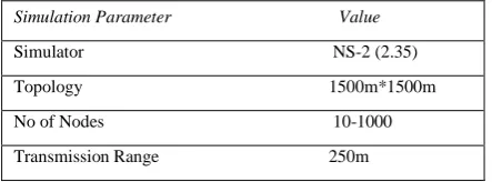
Table: 1 Simulation Parameters
Simulation Parameter Value
Simulator NS-2 (2.35)
Topology 1500m*1500m
No of Nodes 10-1000
Transmission Range 250m
Bandwidth 3 Mbps
Queue Length 50
Packet Size 1040
Pause Time 0s
Min Speed 1 m/s
Max Speed 10-100 m/s
Simulation Time 120s
Routing Protocols DSR,AODV,DSDV
. In Performance evaluation, simulation conducted on two types of topologies. They are fixed topology and Random topology. Random topology means all the nodes placed randomly on different simulation runs. Fixed topology means node position are similar on any simulation run.
4. SIMULATION RESULTS
In this Section simulation results are presented. Here, simulations are carried on three protocols i.e. DSR, AODV and DSDV .These protocols performance evaluated by using the following metrics.
1. Packet Delivery Ratio: Packet Delivery Ratio (PDR)
is defined as the total no of packets successfully received by the destination to the no of packets sent by the source.PDR= Number of Packets Received (ACK)/ Number of Packets Sent (TCP).
[image:2.595.320.525.519.640.2]The PDR specifies the performance of protocol that how successfully the packets have been transferred. Larger values give better results. Simulation results specifies that in case of both fixed and random topologies, noticed that AODV out performs DSR and DSDV in almost all the scenarios shown in figure 1 and figure 2. It has been concluded that performance of DSR and DSDV decreases with the increasing no of nodes as DSR and DSDV designed for up to 100 nodes. In case of large networks including both topologies, PDR value is very low. This indicates that DSR and DSDV not suitable for large networks
[image:2.595.52.274.677.759.2]Figure 2: Packet Delivery Ratio of Random network topology
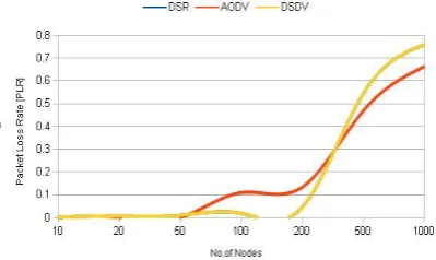
2. Packet Loss Ratio:
Packet Loss Ratio (PLR) is a [image:3.595.326.526.79.198.2]crucial variable for all applications. A high loss rate degrades the communication quality of non-reliable protocols (e.g. for voice or video applications). With reliable transfer protocols, it potentially forces a high number of retransmissions, slows down communication and reduces the usable bandwidth.
Figure 3: Packet Loss Ratio of Fixed network topology
It is defined as the difference between the no of packets sent by the source and received by the sink. In simulation packet loss rate can be calculated at network layer as well as MAC layer. The routing protocol forwards the packet to destination if a valid route is known; otherwise it is buffered until a route is available. There are two cases when a packet is dropped: the buffer is full when the packet needs to be buffered and the time exceeds the limit when the packet has been buffered. Lower values of PLR indicated better performance of the protocol. In case fixed topology AODV has less Packet Loss Ratio shown in figure 3.When network size increases the major packets lost in DSR and DSDV. In case of random topology, the network contains 50 nodes, the performance of all protocols are similar. When network size increases the packet loss rate is high shown in figure 4. This figure also specifies that, AODV slightly low packet loss when compared to DSR and DSDV
3.Routing Overhead :Routing overhead is defined as the
ratio of total no of routing packets to the data packets which has been calculated at the MAC layer.Figure 4: Packet Loss Ratio of random network topology
[image:3.595.325.529.299.429.2]Simulation results show that, in both topologies routing overhead is negligible when network is minimal. The simulation result also specifies performance of DSDV is poor compare with other protocols shown in figures 5 and 6. These results show that a large network creates more routing overhead
Figure 5: Routing overhead of fixed network topology
4. Throughput:
Network throughput is the one of mostimportant parameter to evaluate the performance of wireless mesh networks. High throughput values are desired
[image:3.595.59.286.310.430.2]Throughput is defined as the total no of bits delivered by total duration of simulation time. In fixed topology, AODV achieves high throughput value. When network size is 100, the performances of protocols are same .When network size increases the data rate of DSR and DSDV drops to below 50 kbps shown in figure 7.
[image:3.595.323.532.568.660.2]Figure 7 Throughput of fixed network topology
In case of Random topology, AODV has better value when compared to DSR and DSDV. When network size is 50, the performances of protocols are same. When network size increases, the throughput of DSR and DSDV drops down to zero. This result indicates those protocols are not sufficient for large networks.
[image:4.595.322.526.78.179.2]5. Hop Count: It is defined as the number of hops between
the source and destination of a path. It ignores issues such as link load and link quality. Hop count tends to select long distance links with low quality, which typically already operate at the lowest possible rate, due the link layer’s auto rate mechanismFigure 8: Throughput of Random network topology
Figure 9: Dependencies of the hop count metric [4]
[image:4.595.322.529.256.381.2]Hop count can be dependent on interference and placement in the scenarios of mobility, hop count can out-perform other load dependent metrics shown in figure 9. This is mostly a result of the metric’s agility. Hop count is also a metric with high stability and further has the isotonicity property, which allows minimum weight paths to be found efficiently.
Figure 10 Hop Count of Fixed Topology
[image:4.595.66.267.367.490.2]Simulation result shows that, all routing protocols having same hop count in most of the cases shown in figure 10 and 11. It indicates that node mobility is minimal in mesh networks.
Figure 11 Hop Count of Random Topology
Hop count metric choose paths with low throughput and cause poor medium utilization, as slower links will take more time to send packets. Hop count does not take into account of parameters such as link load, link capacity, link quality, channel diversity or other specific node characteristics.
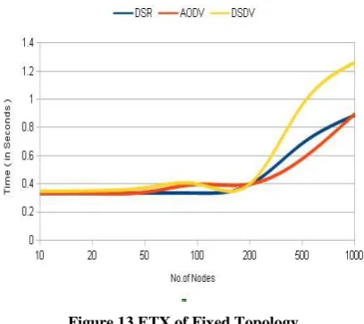
6. ETX:
Expected Transmission Count (ETX) is defined asthe number of transmissions required to successfully deliver a packet over a wireless link. The ETX path metric is simply the sum of the ETX values of the individual links. ETX is a measure of link and path quality.
The ETX metric for a single link is defined as shown below, where df is the measured rate or probability that a packet will be successfully delivered in the forward direction and dr denotes the probability that the corresponding acknowledgement packet is successfully received.
ETX=1/ (df×dr)
[image:4.595.65.269.537.622.2] [image:4.595.332.521.598.747.2]ETX is mostly determined by means of active probing, in which the number of successfully received packets is compared with the number of packets sent in a given time window, which is typically around 10 seconds.
Figure 13 ETX of Fixed Topology
[image:5.595.333.536.214.342.2]Simulation results show that in case of fixed topology, ETX value is constant up to network size is up to 50 nodes. When the network size increases, the no required transmissions are more .As shown in figure 13, the performance of DSR and AODV are similar at 1000 nodes .The Performance of DSDV algorithm is very poor when network size is large and it takes four times of data transfer.
Figure 14 ETX of Random Topology
In random topology, the expected transmissions are similar to at network size 100. The performance of AODV is better than DSR and DSDV when network size increases. When network size is 1000, the expected transmissions are thrice to send packets in case of DSR and DSDV as shown in figure 14.
While ETX outperforms hop count in single-radio and single-rate networks, it does not perform well in multi-rate and multi-radio networks due to its lack of knowledge of co channel interference and its insensitivity to different link rates or capacities.
ETX does not consider the load of a link and will therefore route through heavily loaded nodes without due consideration, leading to unbalanced resource usage. ETX does not discriminate between node types and makes no attempt to minimize intra-flow interference by choosing channel-diverse paths.
7. ETT:
The Expected transmission time (ETT) metric is anextension of ETX which considers different link routes or capacities. ETT is simply the expected time to successfully transmit a packet at the MAC layer and is defined as follows for a single link:
ETT=ETX×(S/B)
[image:5.595.308.537.266.743.2]S denotes the average size of a packet and B the current link bandwidth. The ETT path metric is obtained by adding up all the ETT values of the individual links in the path. Low ETT values are desired.
Figure 15 Dependencies of the ETT metric [4]
:
Figure 16: ETT of Fixed Topology
[image:5.595.62.267.403.533.2]In fixed topology, simulation results shows that, ETT value (in m seconds) is constant at network size is 50. Increasing the network size, ETT value also increases .The performance of DSR and AODV are Similar at network size is 1000.When network size increases, the ETT of DSDV also increases shown in figure 16.In random topology, the simulation results shows that the ETT values are similar at network size is 100.When network size increases the performance of AODV and DSR are better than DSDV shown in figure 17.ETT retains many of the properties of ETX.ETT still does not consider link load explicitly and therefore cannot avoid routing traffic through already heavily loaded nodes and links. ETT was not designed for multi-radio networks and therefore does not attempt to minimize intra-flow interference.
5. CONCLUSION
Routing Protocol is an important component of Communication in Wireless Mesh Networks. Metric is the important measurement of routing protocol. In this paper routing protocols are described. The performance evaluation and investigations are carried out on acquired simulation results of three prominent protocols, AODV, DSR and DSDV. DSDV is selected as representative of proactive routing protocol while AODV and DSR is the representative of reactive routing protocols. As AODV is designed for up to thousands of nodes while DSR is designed up to two hundred nodes. AODV and DSR are proved to be better than DSDV. While it is not very clear that any one protocol is best for all the scenarios, each protocol is having its own advantages and disadvantages and may be well suited for certain scenarios.
These metric based evaluations have been presented, highlighting their features and problems, in order to provide a better understanding of the research challenges of routing protocols for Wireless Mesh Networks.
6. REFERENCES
[1] Y. Yang, J. Wang, and R. Kravets, "Designing Routing Metrics forMesh Networks," IEEE Workshop on Wireless Mesh Networks (WiMesh),Proceedings of the, June 2005.
[2] Sonia Waharte, Raouf Boutaba, Youssef Iraqi, Brent Ishibashi, Routing protocols in wireless mesh networks: challenges and design considerations
[3] J. Broch, D. B. Johnson, D. A. Maltz, The Dynamic Source Routing Protocol for Mobile Ad Hoc Networks," IETF Internet Draft draft-ietf-manet-dsr-01.txt, December 1998
[4] Rainer Baumann, Simon Heimlicher, Mario Strasser, Andreas Weibel, “A Survey on Routing Metrics”. February 10, 2007
[5] S.S.Tyagi and R.K.Chauhan “Performance Analysis of proactive and reactive routing protocols for Adhoc Networks”.
[6] C. E. Perkins and E. M. Royer, Ad-hoc On-Demand Distance Vector Routing," Proceedings of 2nd IEEE Workshop on Mobile Computing Systems and Applications, February 1999.
[7] S. Siva Nageswara Rao, Y. K. Sundara Krishna, and K.Nageswara Rao,“A Survey: Routing Protocols for Wireless Mesh Networks”, IJRRWSN Vol. 1, No. 3.
[8] S. Siva Nageswara Rao, Y. K. Sundara Krishna, and K.Nageswara Rao: A Study of Routing Metrics for Wireless Mesh Networks.