http://dx.doi.org/10.4236/am.2014.513195
How to cite this paper: Tamba, J.G., Koffi, F.D., Lissouck, M., Ndame, M. and Afuoti, N.E. (2014) A Trivariate Causality Test: A Case Study in Cameroon. Applied Mathematics, 5, 2028-2033. http://dx.doi.org/10.4236/am.2014.513195
A Trivariate Causality Test: A Case Study in
Cameroon
Jean Gaston Tamba*, Francis Djanna Koffi, Michel Lissouck, Max Ndame,
Ngwa Engelbert Afuoti
Department of Thermal and Energy Engineering, University Institute of Technology, University of Douala, Douala, Cameroon
Email: [email protected]
Received 7 April 2014; revised 21 May 2014; accepted 1 June 2014
Copyright © 2014 by authors and Scientific Research Publishing Inc.
This work is licensed under the Creative Commons Attribution International License (CC BY). http://creativecommons.org/licenses/by/4.0/
Abstract
In this paper, we examine the causal relationship between diesel consumption, CO2 emissions and
GDP in Cameroon during the period 1975-2008. Cointegration and vector error-correction model-ling techniques are used in this study. ADF tests show that the series, after logarithmic transfor-mation, are non-stationary and integrated of order one. This study finds the presence of a long-run equilibrium relationship between the variables. The results of the Granger-causality tests for time series have been estimated.
Keywords
Causality, Coitegration, VECM, Cameroon
1. Introduction
According to Ghosh [1] and Omri [2], there have been three streams of research to investigate the causal rela-tionship between carbon dioxide emissions, energy consumption and economic growth. Investigating the causal relationship between economic growth and environmental pollutants constitutes the first stream of research. Here, researchers study the existence of environmental Kuznets curve [3] [4]. The causal relationship between energy consumption and economic growth is the second stream of research. This relationship suggests that energy con-sumption and economic growth may be jointly determined and the direction of causality may not be determined a priori. Starting with the work of Kraft and Kraft [5], a number of studies examine the causal relationship be-tween energy consumption and economic growth [6] [7]. Finally, the last stream of research has emerged in the recent literature, which combines two approaches earlier by examining dynamic relationship between CO2
sions, energy consumption and economic growth. The analysis of the causal relationship between CO2 emissions,
energy consumption and economic growth has been subject to many empirical studies [2] [8] [9].
This study has been carried out on various samples of countries. This research shows that there is no clear conclusion about energy consumption, environmental pollutants and economic growth. We note that a wide range of econometric techniques and procedures have been used to test the validity of the relation between en-vironmental pollutants, energy consumption and economic growth. The results and implications of these studies clearly depend on the underlying variables, data frequency, and the development stages of a country [8]. Thus, we remark that conclusion of these studies is various.
To date, no study has been carried out on the causal relationship between CO2 emissions, energy (or diesel)
consumption and economic growth in Cameroon. The aims of this paper are therefore to describe the relation-ship between total CO2 emissions, diesel consumption and economic growth, and to investigate the long run and
short run causality relationship based on the VECM between total CO2 emissions, diesel consumption and GDP
from 1975 to 2008 in Cameroon.
The remainder of this paper is organized as follows: the next section presents an overview of the proposed methodology and data descriptions. In Section 3, the empirical results are reported and the last section concludes the study.
2. Methodology and Data Descriptions
According to Engle and Granger [10], the series x and y of a non-stationary linear combination (with the same order of integration) may be stationary. If such a stationary linear combination exists, the variables are considered to be cointegrated. However, the variables may have the property that a particular combination is sta-tionary. The linear combination can be written as follows Equation (1).
t t t
z = − −x a by (1)
where a and b are two constants term such that the variable zt is stationary, xt and yt will tend to vary together with time and can be subjected to temporary diversions, but cannot diverge without limit. Equation (1) is a long-run equilibrium relationship and zt measures the deviation with respect to the equilibrium value.
The first step tests for the order of integration of the natural logarithm of the variables using Augmented Di- ckey-Fuller (ADF) [11]. For the time series xt, ADF relationship is expressed as:
(
1)
1 1k j
t t j t j t
x α ρ x− =θ x− ε
∆ = + − +
∑
∆ + . (2)where ∆ is the difference operator, k is the auto-regressive lag length and α and ρ are the coefficients of interest. When these series are found to be non-stationary, we take first-difference and we apply the ADF tests again on the differenced data and so on.
The second step involves examining cointegration relationship among the variables using vector autoregres-sive (VAR) approach of Johansen [12] [13] and Johansen and Juselius [14]. We determine the number of long- run equilibrium relationships between integrated variables of the same order. Let xt be a vector variables inte-grated of order one of dimension p×1. The representation VAR of order k is given by:
1 1 0 1
t t k t k t
x = Πx− + + Π x− +µ +µt+ε . (3)
where Π1,,Πk are
(
p×p)
lag coefficient matrices, εt is a(
p×1)
vector of disturbance terms assumed normal and independent with zero mean and non-singular variance-covariance matrix. µ0 and µ1 are(
p×1)
vector of constants terms and trends terms respectively. We can rewrite this structural VAR in error form as:
1
1 1 0 1
k
t t i i t i t
x x− =− x− µ µt ε
∆ = Π +
∑
Γ ∆ + + + . (4)where Γ = − − Π − − Π Π = − − Π − − Πi
(
I 1 i)
,(
I 1 k)
and i=1,,k−1.By examining the Π matrix, we can detect the existence of cointegrating relationship among the x variables. If the rank
( )
r of Π,r=0,∆xt is stationary and all linear combination of xt are integrated of order one. If r=n, all variables xt are stationary. The most interesting case is 0< <r n, where r and n denote the rank offormally tested with two common approaches, namely the maximum eigenvalue test and the trace test. The like-lihood ratio statistics for the maximum eigenvalue test and the trace test are Equations (5) and (6) respectively:
(
*)
max Tlog 1 r 1
λ = − −λ+ . (5)
(
)
1
*
Trace p log 1
i r= +T λi
= −
∑
− . (6)where T is the maximum time in the time series t. Since the cointegration tests are sensitive to the choice of lag length, we use the Schwartz Information Criteria (SIC) to determine the optimal lag lengths.
Cointegration implies that causality exists between the series, but it does not indicate the direction of the causal relationship [6]. Therefore, we use the VECM to detect the direction of the causality. The causality based on the VECM has the advantage of giving a causal relationship even without any significant estimated coeffi-cients [15]. Granger [16] sustains that if variables are non-stationary, but become stationary after the difference, and cointegrated, it becomes necessary to estimate a VECM for the multivariate causality test. The VECMs for this test can be specified accordingly as Ang [17], Ang [18], Odhiambo [19] and Ghosh [1]:
10 1 11 1 12 1 13 14ECT 1 1
p p
t i t i i i t i i i t i t
p
i t
x β =β x− = β y− = β z− β − µ
∆ = +
∑
∆ +∑
∆ +∑
∆ + + . (7)20 1 21 1 22 1 23 24ECT 1 2
p p p
t i i t i i i t i i i t i t t
y β = β y− = β x− =β z− β − µ
∆ = +
∑
∆ +∑
∆ +∑
∆ + + (8)30 1 31 1 32 1 33 34ECT 1 3
p p p
t i i t i i i t i i i t i t t
z β = β z− = β y− = β x− β − µ
∆ = +
∑
∆ +∑
∆ +∑
∆ + + (9)where xt, yt and zt represent CO2 emissions, diesel consumption and economic growth in logarithmic form
respectively. ∆ is the difference operator, β s are the parameters to be estimated and µt are the serially un-correlated error terms. ECTt−1 is the error correction term, which is derived from long run cointegration
rela-tionship. In the Wald tests, chi-square χ2
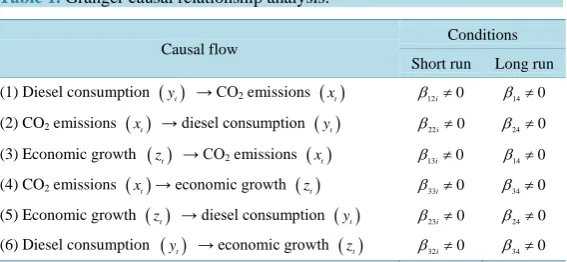
statistics and their probabilities were obtained to determine the short run causalities in VECM [17] [18]. The t-statistics on the coefficients of the lagged error-correction term indi-cates the significance of the long run causal effect [1] [19]. The optimum lag length p is determined on the ba- sis of SC. In our study the Granger causal relationship analysis is given in Table 1 [19].
Our empirical study uses the time data of CO2 emissions, diesel consumption and GDP for the 1975-2008
pe-riod in Cameroon. In this paper, CO2 emissions measured by a metric tons CO2 and data are obtained from the
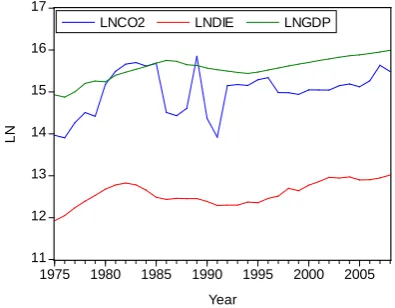
World Development Indicators produced by the World Bank [20]. Diesel consumption and GDP are taken in Tamba et al.[6]. The logarithm terms of these variables are used because the logarithmic transformation leads to a more stable variance of data. LNCO2 is the logarithm of CO2 emissions, LNDIE is the logarithm of diesel
consumption and LNGDP is the logarithm of GDP. The GDP is used as a proxy for economic growth. Figure 1
shows logarithmic transformation of the evolution of total CO2 emissions, diesel consumption and development
of Cameroon’s GDP from 1975 to 2008.
3. Empirical Results
The results of the ADF tests on the integration properties of the CO2 emissions, diesel consumption and GDP for
[image:3.595.156.440.591.722.2]Cameroon indicate that the series are stationary in first difference. This shows that the LNCO2, LNDIE and LNGDP variables are individually integrated of order one.
Table 1.Granger causal relationship analysis.
Causal flow Conditions
Short run Long run
The cointegration analysis is typically applied to verify if there exists a long run relationship between the variables. The results of the Johansen maximum likelihood cointegration tests are presented in Table 2. Table 2
presents maximum eigenvalues and trace statistics and shows the cointegration relationship among variables. The number of cointegration test is two according to the trace test and one by the maximum eigenvalue test at the 5% significance level. In this paper, we are only interested in the first cointegrating equation because of its ability to determine the impact of the explicative variables under consideration of the CO2 emissions in the long
run. Therefore, we use the maximum eigenvalue tests.
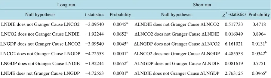
Cointegration implies the existence of Granger-causality but it does not indicate the direction on the causality relationship. The multivariate Granger-causality tests based on the VECM are carried out to examine both long run and short run causality. The results of the Granger-causality tests for time series based on the VECM are shown in Table 3. the results confirm the unidirectional long run causality and no causality in the short run rela-tionship between total CO2 emissions and diesel consumption, both the bidirectional long run and short run
cau-sality relationship between total CO2 emissions and GDP, and the unidirectional long run causality and no
cau-sality in the short run relationship between diesel consumption and GDP at the 5% level of significance in Cam-eroon.
4. Conclusions and Policy Implications
This paper analyses the causal relationship between total CO2 emissions, diesel consumption and GDP in
[image:4.595.214.412.368.522.2]Cam-eroon over the period 1975-2008. We began by testing the order of integration of series by the ADF unit root test. Then we tested the Johansen multivariate cointegration to determine the existence of a long run relationship between variables. Finally, Granger-causality tests based on the VECM were employed. VECM tests were used to estimate the direction of Granger-causality for the multivariate cointegration data.
Figure 1.Logarithmic transformation of the variables from 1975 to 2008.
Table 2.Johansen and Juselius cointegration test.
Number of cointegration Eigenvalue Statistic 5% Critical value Probabilityb
Trace test
Nonea 0.640165 55.34624 35.19275 0.0001
At most 1a 0.391305 22.63873 20.26184 0.0231
At most 2 0.190245 6.752740 9.164546 0.1401
Maximum eigenvalue test
Nonea 0.640165 32.70751 22.29962 0.0013
At most 1 0.391305 15.88599 15.89210 0.0501
At most 2 0.190245 6.752740 9.164546 0.1401
a
denotes rejection of the hypothesis at the 5% significance level; bMacKinnon-Haug-Michelis (1999) p-values.
11 12 13 14 15 16 17
1975 1980 1985 1990 1995 2000 2005
LNCO2 LNDIE LNGDP
Year
L
[image:4.595.89.542.572.709.2]Table 3.Granger-causality test for time series based on the VECM.
Long run Short run
Null hypothesis t-statistics Probability Null hypothesis: χ2
-statistics Probability
LNDIE does not Granger Cause LNCO2 −3.09540 0.0045a ΔLNDIE does not Granger Cause ΔLNCO2 0.517733 0.4718
LNCO2 does not Granger Cause LNDIE −1.92244 0.0652c ΔLNCO2 does not Granger Cause ΔLNDIE 0.016949 0.8964
LNGDP does not Granger Cause LNCO2 −3.09540 0.0045a ΔLNGDP does not Granger Cause ΔLNCO2 6.161021 0.0131b
LNCO2 does not Granger Cause LNGDP −4.72553 0.0001a ΔLNCO2 does not Granger Cause ΔLNGDP 4.485553 0.0342b
LNGDP does not Granger Cause LNDIE −1.92244 0.0652c ΔLNGDP does not Granger Cause ΔLNDIE 0.081619 0.7751
LNDIE does not Granger Cause LNGDP −4.72553 0.0001a ΔLNDIE does not Granger Cause ΔLNGDP 2.763125 0.0965c
a
Denotes significance level at 1%; bDenotes significance level at 5%; cDenotes significance level at 10% respectively.
The results indicate that the time series are in first stationary difference. The Johansen multivariate cointegra-tion tests concluded the existence of a long-run relacointegra-tionship between the variables. The Granger-causality tests based on the VECM show that there exist: (1) unidirectional and bidirectional causality between the variables in the long run and (2) no causality and bidirectional causality between the variables in the short run at the 5% le- vel of significance.
In Cameroon, a government policy aimed at improving energy supply and economic growth will inevitably have a positive impact on total CO2 emissions from an environmental point of view. That is, “reinforce
Camer-oon energy demands with low emission fuel and respect the terms of the UNFCCC by mitigating emissions while ameliorating economic growth”. Hence, GDP growth and energy consumption will stimulate total CO2
emissions.
References
[1] Ghosh, S. (2010) Examining Carbon Emissions Economic Growth Nexus for India: A Multivariate Cointegration Ap-proach. Energy Policy, 38, 3008-3014. http://dx.doi.org/10.1016/j.enpol.2010.01.040
[2] Omri, A. (2013) CO2 Emissions, Energy Consumption and Economic Growth Nexus in Mena Countries: Evidence
from Simultaneous Equations Models. Energy Economics, 40, 657-664. http://dx.doi.org/10.1016/j.eneco.2013.09.003
[3] Stern, D. (2004) The Rise and Fall of the Environmental Kuznets Curve. World Development, 32, 1419-1439.
http://dx.doi.org/10.1016/j.worlddev.2004.03.004
[4] Dinda, S. (2004) Environmental Kuznets Curve Hypothesis: A Survey. Ecological Economics, 49, 431-455.
http://dx.doi.org/10.1016/j.ecolecon.2004.02.011
[5] Kraft, J. and Kraft, A. (1987) On the Relationship between Energy and GNP. Journal of Energy and Development, 3, 401-403.
[6] Tamba, J.G., Njomo, D., Limanond, T. and Ntsafack, B. (2012) Causality Analysis of Diesel Consumption and Econo- mic Growth in Cameroon. Energy Policy, 45, 567-575. http://dx.doi.org/10.1016/j.enpol.2012.03.006
[7] Fondja Wandji, Y.D. (2013) Energy Consumption and Economic Growth: Evidence from Cameroon. Energy Policy, 61, 1295-1304. http://dx.doi.org/10.1016/j.enpol.2013.05.115
[8] Lotfalipour, M.R., Falahi, M.A. and Ashena, M. (2010) Economic Growth, CO2 Emissions, and Fossil Fuels Consump-
tion in Iran. Energy, 35, 5115-5120. http://dx.doi.org/10.1016/j.energy.2010.08.004
[9] Chandran Govindaraju, V.G.R. and Tang, C.F. (2013) The Dynamic Links between CO2 Emissions, Economic Growth
and Coal Consumption in China and India. Applied Energy, 104, 310-318.
http://dx.doi.org/10.1016/j.apenergy.2012.10.042
[10] Engle, R.F. and Granger, C.W.J. (1987) Co-Integration and Error Correction: Representation Estimation and Testing.
Econometrica, 55, 251-276. http://dx.doi.org/10.2307/1913236
[11] Dickey, D.A. and Fuller, W.A. (1981) Likelihood Ratio Statistics for Autoregressive Time Series with a Unit Root.
Econometrica, 49, 1057-1072. http://dx.doi.org/10.2307/1912517
[12] Johansen, S. (1988) Statistical Analysis of Cointegrating Vectors. Journal of Economic Dynamics and Control, 12, 231-254. http://dx.doi.org/10.1016/0165-1889(88)90041-3
Models. Econometrica, 59, 1551-1580. http://dx.doi.org/10.2307/2938278
[14] Johansen, S. and Juselius, K. (1990) Maximum Likelihood Estimation and Inferences on Cointegration with Applica-tion to the Demand for Money. Oxford Bulletin of Economics and Statistics, 52, 169-210.
http://dx.doi.org/10.1111/j.1468-0084.1990.mp52002003.x
[15] Belloumi, M. (2009) Energy Consumption and GDP in Tunisia: Cointegration and Causality Analysis. Energy Policy, 37, 2745-2753. http://dx.doi.org/10.1016/j.enpol.2009.03.027
[16] Granger, C.W.J. (1988) Some Recent Developments in Concept of Causality. Journal of Econometrics, 39, 199-211.
http://dx.doi.org/10.1016/0304-4076(88)90045-0
[17] Ang, J.B. (2007) CO2 Emissions, Energy Consumption, and Output in France. Energy Policy, 35, 4772-4778.
http://dx.doi.org/10.1016/j.enpol.2007.03.032
[18] Ang, J.B. (2008) Economic Development, Pollutant Emissions and Energy Consumption in Malaysia. Journal of Poli-cy Modeling, 30, 271-278. http://dx.doi.org/10.1016/j.jpolmod.2007.04.010
[19] Odhiambo, N.M. (2009) Electricity Consumption and Economic Growth in South Africa: A Trivariate Causality Test.
Energy Economics, 31, 635-640. http://dx.doi.org/10.1016/j.eneco.2009.01.005
currently publishing more than 200 open access, online, peer-reviewed journals covering a wide range of academic disciplines. SCIRP serves the worldwide academic communities and contributes to the progress and application of science with its publication.