Analysis of Hopfield Associative Memory with
Combination of MC Adaptation Rule and an Evolutionary
Algorithm
Amit Singh
Asst. Professor Sharda University Greater Noida, UP, INDIA
Somesh Kumar
Professor
Noida Inst. Of Engg. & Tech. Greater Noida, UP, INDIA
T. P. Singh
Asst. Professor Sharda University Greater Noida, UP, INDIA
ABSTRACT
The combination of evolutionary algorithms and ANN has been a recent interest in the field of research. Hopfield model is a type of recurrent neural network which has been widely studied for the purpose of associative memories. In the present work, this Hopfield Model of feedback neural networks has been studied with Monte Carlo adaptation learning rule and one evolutionary searching algorithm i.e. genetic algorithm for pattern association. The aim is to obtain the optimal weight matrices with the MC-adaptation rule and Genetic algorithm for efficient recalling of any approximate input patterns. The experiments consider the Hopfield neural networks architectures that store all objects using Monte Carlo-adaptation rule and simulates the recalling of these stored patterns on presentation of prototype input patterns using evolutionary algorithm (Genetic Algorithm). Experiment shows the recalling of patterns using genetic algorithm have better results than the conventional recalling with Hebbian rule.
General Terms
Pattern Association, Hopfield Neural Network, Monte Carlo-adaptation Rule and Evolutionary Algorithm.
Keywords
Hopfield Neural Network with associative memory for pattern association problem using MC-adaptation rule and Evolutionary Genetic Algorithm.
1.
INTRODUCTION
There are numerous examples which demonstrate that a human brain can learn, understand and remember certain things completely, partially and sometimes not at all. Most of the children of five-year age group can start recognizing digits, letters, shapes, objects etc. either hand drawn, machine printed, or rotated. Depending on our capacity for learning, the information is stored in our brain [1][2][3].The inherent differences in information handling by human beings and machines are in the form of patterns and data, and also their functions of understanding and recognizing.
Pattern association is a salient feature of human memory. Associative memory models, known as content-addressable memories, are class of the most extensively analyzed in neural networks. Associative memories can be either heteroassociative or autoassociative. It involves storing a set of patterns or a set of input-output pattern pairs in such a way that when test data are presented, the pattern or pattern pair corresponding to the data is recalled. This is purely a memory function to be performed for patterns [4][5][6].
The main characteristics of neural networks are that they have
relationships, use sequential training procedures, and adapt themselves to the data. Artificial neural Networks specially, Hopfield type are very good candidates for solving pattern association problems [7][8].
2.
BACKGROUND WORK
Weight training in ANN's is usually formulated as minimization of an error function, such as the mean square error between target and actual outputs averaged over all examples, by iteratively adjusting connection weights. Most training algorithms, such as Back Propagation (BP) and conjugate gradient algorithms [9] are based on gradient descent. There have been some successful applications of BP in various areas [10], but BP has drawbacks due to its use of gradient descent. It often gets trapped in a local minimum of the error function and is incapable of finding a global minimum if the error function is multimodal and/or non-differentiable. A detailed review of BP and other learning algorithms can be found in [11].
One way to overcome gradient-descent-based training algorithms' shortcomings is to formulate the training process as the evolution of connection weights in the environment determined by the architecture and the learning task. Evolutionary algorithms [12][15-16] can then be used effectively in the evolution to find a near-optimal set of connection weights globally without computing gradient information. The fitness of an ANN can be defined according to different needs.
The performance of the Hopfield neural networks, especially the quality of recall and the capacity of the effective storing, can be greatly improved by making use of a neural network designing method without altering whole structure of the network. By the use of genetic algorithm [17][18][19] with MC-adaptation rule [20], one can avoid applying the overlap criterion as carried out in the Hopfield neural network with conventional Hebbian rule.
3.
HOPFIELD NEURAL NETWORK
A HNN is a simple recurrent type artificial neural network which is able to store certain memories or patterns in a manner rather similar to the brain - the full pattern can be recovered if the network is presented with only partial information about stored patterns [13][14].
"closest" to the starting pattern. In other words, we can give the network a corrupted image or memory and the network will "all by itself" try to reconstruct the perfect image.
In HNN, the output of each unit is fed to all the other units with weights wij except wii, let the output function of each of the units be bipolar so that
where is the threshold for the unit i.
The state of each unit is either +1 or –1 at any given instant of time. The state at time (t+1) is the same as the state at time (t) for all the units. That is,
for all i
Associated with each state of the network, Hopfield proposed an energy function whose values always either reduces or remains the same as the state of the network changes. Assuming the threshold value of the unit i to be , the energy function is given by
The energy as a function of the state of the network describes the energy landscape in the state space. The energy landscape is determined only by the network architecture, i.e., the number of units, their output functions, threshold values, connections between units and the strengths of the connections.
The change in energy due to update of the kth unit is given by
And therefore,
Therefore the energy decreases or remains the same when a unit, selected at random, is updated provided the weights are symmetric, and the self-feedback is zero.
3.1
Hebbian Rule
Synaptic dynamics, as discussed earlier, is described in terms of expressions for the first derivative of the weights. They are called learning equations. The proposed Hopfield model consists of N neurons and N2 connection strengths.
Hebbian is the simplest learning rule, in which each neuron can be in one of the two states, i.e. ±1, and p bipolar patterns
X are to be
memorized in associative memory. In this type of neural network, the coupling matrix is usually determined by the Hebbian rule as follows:
x
i is representing the ith bit of µth pattern. where i = 1,2 …..N (number of bits in a pattern) and µ = 1,2 …..p (number of patterns)3.2
MC-Adaptation Rule
The MC-adaptation rule [21] is different from the conventional Hebbian rule as well as other learning rules such as perceptron. It has been shown that, by applying this rule, one can design neural networks with controllable degree of symmetry. When apply this rules memory patterns are input into the learning process one by one. i.e. each time the adaptation of the coupling matrix is carried out by pursuing the optimal solution for a specific memory pattern. Hebbian is local learning rule while MC-adaptation rule is a global design rule.
Most of the time for the application of MC-adaptation rule in HNN, we generally initialize the coupling matrix using Hebbian rule but in this paper we have changed the initial weight matrix by random weight matrix as given below in the first step.
Step 1:
Coupling matrix can be obtained randomly with four digit decimal numbers between -1 and 1. Then we apply the MC adaptation rule to guarantee all the memory patterns satisfying the fixed point condition by driving the local fields to the region of the following:
Where
Step 2:
Specify a row in the coupling matrix , say the ith row, and calculate:
For and (patterns)
Step 3:
Now find the ) and let record the
indices of patterns satisfying
Step 4:
Initialize two variables as:
and proceed as:
if
otherwise
Step 5:
Now, record column indices with
satisfying condition and
with satisfying condition respectively.
Step 6:
Adaptation follows as:
If randomly pick j form the list
and make adaptation
If randomly pick j from the list and make adaptation
Otherwise randomly pick an index from the list
or with equal
probability, and if make an
adaptation
Otherwise
Repeat Step 2 to Step 6 until
Apply the above procedure until for all rows.
After executing algorithm for all rows (i), we will obtain a desirable optimal weight matrix J with the patterns being memory as fixed point.
4.
THE GENETIC ALGORITHM
Thus, ANN and genetic algorithms are two techniques for optimization and learning, each with its own strength and weaknesses. The two have generally evolved along separate paths. However, recently there have been attempts to combine the two technologies and researchers have combined neural network and genetic algorithms in a number of different ways
In this simulation, recalling is done by Genetic Algorithm. When GA [22-23] starts, a population of weight matrices is produced by crossover from the parent weight matrices which are generated by MC adaptation rule in the storing stage. In each generation, this population is modified through uniform random mutations and their fitness values are evaluated.
The cycle of generating the new population with better individuals and restarting the search is repeated until an optimum solution was found. The fitness function is
evaluating the best matrices of the weights population on the basics of the hundred percent successful recalling with zero bit error of the stored patterns on the presentation of the same as the input pattern. It indicates that the stable states of the network will be used for the evaluation of the weight’s population.
Crossover generates new population of size:
N*N + Initial population,
where N is number of neuron.
Fitness function evaluates and collect all those weight matrices which can successfully recall the respective stored patterns by providing the same as input pattern (with no error) at a time will be considered as fitted weight matrix.
After fitness evaluation mutation operator executes to increase the population and generates population of size:
N*N + Fitted Population
Now this generated population will be used for recalling purpose.
5.
EXPERIMENTS
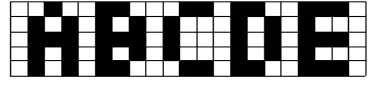
[image:3.595.334.521.377.422.2]The patterns used for the simulations are shown in Figure 1. Each pattern consisted of a 5 X 3 pixel matrix representing an alphabet of the set. White and black pixels are respectively assigned corresponding values of -1 and +1.
Fig 1: Set of patterns used for training
Using these bipolar values, the set of above alphabets is represented in the form a series. For example, object is written as:
[-1 1 -1 1 -1 1 1 1 1 1 -1 1 1 -1 1]
The results presented in this section demonstrate that, within the simulation framework presented above, large significant difference exists between the performance of genetic algorithm conventional Hebbian rule for recalling alphabets those have been stored in Hopfield neural network using MC adaptation rule and Hebbian learning rule respectively.
In total 1000 times the recalling was made through both the algorithms separately for each pattern. In these cases, noise was created by reverting 0-bit, 1-bit, 2-bits and 3-bits in the presented prototype input patterns in the already stored patterns. These positions of the bit(s) to be reverted to create noise are taken randomly.
Table 1: The results of recalling of taken set of alphabets when there is no error in the presented input prototype
patterns Alphabets P att ern 1 P att ern 2 P att ern 3 P att ern 4 P att ern 5 Re ca ll in g S u cc ess (in %) He b b ia n
84.0 100 100 94.3 86.4
[image:4.595.308.556.110.354.2] [image:4.595.45.292.335.575.2]GA 100 100 100 100 100
Table 21: The results of recalling of taken set of alphabets when there is 1-bit error in the presented input prototype
patterns Alphabets P att ern 1 P att ern 2 P att ern 3 P att ern 4 P att ern 5 Re ca ll in g S u cc ess (in %) He b b ia n
5.3 6.0 6.6 5.6 6.5
GA 100 100 100 100 100
Reverted bit
[image:4.595.310.555.375.643.2]position 12 2 5 9 13
Table 22: The results of recalling of taken set of alphabets
when there is 1-bit error in the presented input prototype patterns
* Pattern 4 was recalled instead pattern 2
Alphabets P att ern 1 P att ern 2 P att ern 3 P att ern 4 P att ern 5 Re ca ll in g S u cc ess (in %) He b b ia n 6.5 94.0
(4)* 6.6 5.9 7.1
GA 99.1
100
(4)* 99.2 100 100
Reverted bit
position 3 8 9 10 5
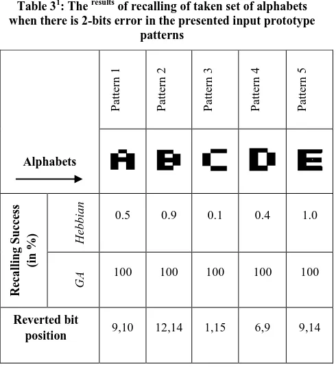
Table 31: The results of recalling of taken set of alphabets when there is 2-bits error in the presented input prototype
patterns Alphabets P att ern 1 P att ern 2 P att ern 3 P att ern 4 P att ern 5 Re ca ll in g S u cc ess (in %) He b b ia n
0.5 0.9 0.1 0.4 1.0
GA
100 100 100 100 100
Reverted bit
Table 32: The results of recalling of taken set of alphabets
when there is 2-bits error in the presented input prototype patterns
* Pattern 2 was recalled instead pattern 4
Alphabets P att ern 1 P att ern 2 P att ern 3 P att ern 4 P att ern 5 Re ca ll in g S u cc ess (in %) H eb b ia n
0.6 0.7 1.4 7.2
(2)* 0.7
GA 99.7 98.4 100 (2)* 100 100
Reverted bit position
2,11 11,12 4,9 2,8 3,9
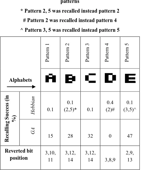
Table 4: The results of recalling of taken set of alphabets when there is 3-bits error in the presented input prototype
patterns
* Pattern 2, 5 was recalled instead pattern 2
# Pattern 2 was recalled instead pattern 4
^ Pattern 3, 5 was recalled instead pattern 5
[image:5.595.48.289.393.682.2]Alphabets P att ern 1 P att ern 2 P att ern 3 P att ern 4 P att ern 5 Re ca ll in g S u cc ess (in %) He b b ia n 0.1 0.1
(2,5)* 0.1 0.4 (2)# 0.1 (3,5)^ G A
15 28 32 0 47
Reverted bit position 3,10, 11 3,12, 14 3,12, 14 3,8,9
2,9, 13
6.
CONCLUSION AND FUTURE SCOPE
By using MC adaptation rule to slightly modify the Hopfield Neural network designed by the Hebbian rule, one can significantly improve the performance of the network. The improved Neural Network has higher storage capacity than
indicating that genetic algorithm with MC adaptation learning rule has more success rate then the Hebbian rule for storing and recalling the taken set of alphabets, which are containing 0, 1, 2, and 3 bit errors from stored patterns in Hopfield neural network. Sometimes it has also been observed that the performance of GA was less than what was expected to be. One of the reason for this deviation may be the position(s) of bits reverted to induce noise in the recalling pattern. Second reason may be high similarity between two stored patterns which can be reduced by taking more pixels and hence more neurons in the Hopfield memory. It is also possible to obtain more than one weight matrices from the generated population of weight matrices as the optimal weight matrices for recalling the exact pattern on presentation of any prototype input pattern of already stored pattern.
The direct application of GA with MC adaptation rule to the pattern association has been explored in this paper. The aim is to introduce as alternative approach to solve the pattern association problem. The results from the experiments conducted on the algorithm are quite encouraging. Nevertheless more work needs to be perform especially on the tests for noisy input patterns. We can extend this concept for pattern recognition for alphabets of different languages, shapes, numerals. Some real dataset of handwritten characters may also be tested using the presented approach and the comparison with the previous approaches may be analyzed.
7.
REFERENCES
[1] Simpson P K, “Foundations of Neural Networks”, Artificial Neural Networks: Paradigms, Applications and Hardware Implementations (E. Sanchez-Sinencio and C. Lau, eds.), New York: IEEE Press, pp. 3-24, 1992.
[2] Anderson J A, Rosenfeld E, “Neurocomputing: Foundations of Research” MIT Press, Boston, MA, 1988.
[3] Hinton G E, Sejnowski T J, “Neural Network Architectures for AI”, Tutorial Number MP2, National Conference on Artificial Intelligence (AAAI-87), July 1987.
[4] Jain A K, Robert P W D, Mao J, “Statistical Pattern Recognition: A Review”, IEEE Transactions on Pattern Analysis and Machine Intelligence, vol. 22, number 1, pp. 4-33, 2000.
[5] Grenander U, General Pattern Theory, Oxford University Press, 1993.
[6] Schalkoft R, Pattern Recognition- Statistical, structural and neural approaches, John Wiley & Sons, 1992.
[7] Kosko, B., “Neural Networks and Fuzzy Systems” Prentice-Hall India, 2005.
[8] Yao X, “Evolving Artificial Neural Network”, Proceedings of the IEEE, vol. 87, number 9, September 1999.
[9] Moller M F, “A scale conjugate gradient algorithm for supervised learning”, Neural Networks, vol 6, number 4, pp 525-533, 1993.
[10]Chauvin Y and Rumelhart D E, Eds., Backpropagation: Theory, Architectures, and Applications, Hillsdale, NJ: Erlbaum, 1995.
Science Society, Hillsdale, NJ: Erbaum, pp. 823 – 831, 1986.
[12]Bremermann H J, “The Evolution of Intelligence: The Nervous System as a Model of its Environment”, Technical Report No. 1, Contract No. 477(17), Department of Mathematics, University of Washigton, Seattle, 1958.
[13]Hopfield J J, “Neurons with graded response have collective computational properties like those of two state neurons”, Proceedings of National Academy of Sciences, vol. 81, pp. 3088-3092, 1984.
[14]Hopfield J J, Tank D W, “Computing with neural circuits: A model”, Science, vol. 233, pp625-633, 1986.
[15]Shapiro J L, “Theoretical aspects of evolutionary computing”, Statistical Mechanics Theory of Genetic Algorithms, Natural Computing (Springer-Verlag, London, UK), pp. 87-108, 2001.
[16]Koza J R and Rice J P, “Genetic generation of both the weights and architecture for a neural network”, in Proceedings of IEEE Int. Joint Conf. Neural Networks (IJCNN'91 Seattle), vol.2, pp. 397-404, 1991.
[17]Wright S, “The evolution of life”, Panel discussion in Evolution After Darwin: Issues in Evolution, vol III, S
Tax and C Callender, Eds. Chicago: University of Chicago Press, 1960.
[18]Bäck T, Hammel U, Schwefel H P, “Evolutionary Computation: Comments on the History and Current State”, IEEE Trans. Evolutionary Computation, vol. 1, pp 3-17, April 1997.
[19]Schaffer J D, Whiltley D and Eshelman, “Combination of genetic algorithm and neural network: The state of the art”, IEEE Computer Society, 1992.
[20]Zhou Zen and Zhao Hong, Improvement in Hopfield Neural Network by MC-adaptation rule, department of physics,Xiamen 2006.
[21]Zhou Zen and Zhao Hong, Improvement in Hopfield Neural Network by MC-adaptation rule, department of physics,Xiamen 2006
[22]A. Imada and K. Araki, (1997) Applications of an Evolutionary Strategy to the Hopfield Model of Associative Memory, in: Proceedings of the IEEE international conference on evolutionary computation, pp. 679-683.