Comparative Analysis of Regression based and
Supervised Learning
Algorithms for Predicting Traffic Noise Levels in
Indian Scenario
Prashant Ruwali Vikas Tripathi
College Of Engineering Roorkee Graphic Era University
ABSTRACT
Road traffic noise has remained one of the greatest concerns during the past few decades.it has found to be the major sources of pollution in the metropolitan city areas [7]. With the increase in urbanization and motorization the number of vehicles has increased which further increased this problem by manifolds. [4] Thus, in view of the above stated problem our aim is perform prediction of noise levels using certain available regression based and supervised learning algorithms. Modelling and prediction of traffic noise by using generally used prediction algorithms is a very complicated and non linear process, due to high involvement of several factors over which noise level depends.[3]. However, after analysis we have been able to found appropriate results with a certain levels of accuracy.
Keywords
Road traffic model (RTM), Artificial neural networks, K-nearest neighbour, Multi linear regression, Polynomial regression, Road traffic, Noise.
1.
INTRODUCTION
Noise is blamed to have negative impact on health. Hearing damage, annoyance, sleep disturbance, high blood pressure ,poor cardiovascular health is all linked to community noise.[2]. In addition, there are various studies carried out on road traffic noise pollution, which results in severe health problems such as, physical and psychological, irritation, human performance and actions [5][14], hypertension, heart problems, tiredness, headache and sore throat respectively [6]. Our earlier works include to perform the modelling of noise using efficient road traffic noise model which we were able to perform with a considerable accuracy [4]. In this paper we put our work to next level by performing prediction of noise levels using various prediction algorithms. As we perform the comparative analysis our aim would be to find results obtained by algorithms such as multi linear regression, polynomial regression, artificial neural networks, k-nearest neighbour then perform analysis of the results obtained by each of the algorithms by calculating the efficiency, different kinds of error between the observed and predicted values and coefficient of correlation 𝑅2. All the data has been acquired from Dehradun-Roorkee highway (NH-58). It comprises of the hourly volume of vehicles (number of vehicles passing through the road annually), percentage of heavy vehicles in the volume of data and observed value of noise [2].The reason of including heavy vehicle percentage is the fact that heavy vehicles play a major role in traffic noise pollution [1]. The observed value of noise is obtained by using noise analyzer (B & K 2260 sound level meter). This sound meter has the capability of measuring measures the level of noise produced in dBA. dBA is approximately
equivalent to the inverse of the 40 dB (at 1 kHz) equal-loudness curve for the human ear. [2][9].
2.
METHODOLOGY
As the work required the usage of four different algorithms which includes Multi linear regression, Polynomial regression, K-nearest neighbour algorithm and artificial neural networks Back propagation. Out of these first two are based on regression while next two belongs to the class of supervised learning algorithms. We would be discussing each of them as follows:
2.1 Multilinear Regression
Multiple regression is basically an extension of linear regression and it basically defines a dependent variable Y depending on two or more independent variables X1, X2, …., Xn. It allows response variable Y to be modelled as a linear function of multidimensional feature vector [13].
The regression line for p different explanatory variables x1, x2, 𝑥3 ... 𝑥𝑝−1 , xp is defined to be
𝛽𝑦 = 𝛼0+𝛼1. 𝑥1+𝛼2𝑥2……… +𝛼𝑝𝑥𝑝.
Where, 𝛼0is the constant term and 𝛼1 to 𝛼𝑝 are the coefficients relating to p explanatory variables
Formally, the model for multiple linear regression, given n observations is
yi = β 0 + β 1xi1 + β2xi2 + ... βpxip + Є i for i = 1,2, ... n.
Errors are assumed independent of the various explanatory variables which is same as that in the linear regression. Moreover, the coefficients are called regression coefficients because they allow for the effect of other variables
Here, in our work we require to use the multi linear regression results because there can be more than one factor on which the noise produced by the road traffic can be depended. In our cases the volume of vehicles at a certain hour of traffic, the time at which data is recorded as the traffic at the peak hours would definitely be greater compared to the traffic at the non peak hours, moreover the percentage of heavy vehicles also play a key role in traffic noise as it is found that the traffic produced by the heavy vehicles is greater compared to the light vehicles.
2.2 Polynomial Regression
more interpretable results which can be easily deducted in terms of possible functional relationships.
𝑌 = 𝑎 + 𝑏1𝑥1+ 𝑏2𝑥2+ 𝑏3𝑥3+………….+𝑏𝑛𝑥𝑛
Even though the problem of fitting polynomial regression is similar to the one of fitting multiple regressions, polynomial regression posses certain features.
We fix polynomial to smooth out fluctuations in the data caused by random or uncontrolled errors, not because it is thought to represent the relationship. While fitting the polynomial regression the form of the null hypothesis takes is that polynomial regression being fitted represents certain relationships and secondly, whether terms of higher degree contributes significantly to the relationship.
In our scenario the polynomial regression is used with two degree as besides increasing the degree does not found to provide any significant results.
In order to solve the polynomial regression equation with two degree it requires converting the equation to the linear form. In order to do so, the transformations obtained are,
𝑋1= 𝑋, 𝑋2= 𝑋2, 𝑋3= 𝑋3,
Thus, the equation obtained by performing this transformation are quite similar to those obtained by multi linear regression which can then be solved by performing method of least square.
2.3 k-Nearest Neighbour Algorithm
KNN is a non parametric lazy learning algorithm. It means is that it does not use the training data points to do any generalization. In other words, there is no explicit training phase or it is very minimal. This means the training phase is pretty fast. Lack of generalization means that KNN keeps all the training data. More exactly, all the training data is needed during the testing phase. Most of the lazy algorithms – especially KNN – make decision based on the entire training data set. These are based on the learning by analogy.
The training samples are described by the n dimensional numeric attribute. Each sample represents point in an n dimensional space. In this way all of the training sample can be are stored in an n dimensional pattern space. When given an unknown sample the k nearest neighbour algorithm searches for the pattern which corresponds to the unknown sample and provide the most appropriate results for it. In order to determine the pattern it defines the closeness of a particular pattern from the unknown sample, and if it is found to be close to each other the unknown sample is classified according to that particular pattern [8]. Now the closeness can be determined by using of the various distance function, but most commonly used is the Euclidean function given by,
ⅆ(𝒙, 𝒚) = ‖𝒙 − 𝒚‖ = √((𝐱 − 𝐲). (𝐱 − 𝐲) ) = ( 𝐱𝐢 − 𝐲𝐢 𝟐
𝐧
𝐢=𝟏
)𝟏/𝟐
The algorithm for performing the k nearest neighbour algorithm is given by:
for j=1:b
for n=j:m
z(n-p)=dist(volume(1,m),volume(1,n));
end [c,index]=sort(z); for k=1:5
h(k)=volume(index(k)); end
predict (1,j)=floor((mean(h)))+1; m=m+1;
volume (1,m)=predict(1,j); p=p+1;
end
Above function predicted ‗b‘ values of 24 hours for the traffic i.e. prediction is made for ‗b‘ days. Thus, by the usage of the above algorithm we calculated all the nearest neighbors which are stored in matrix h on the basis of window size been defined. Mean is calculated of matrix h thus generated, which is then used to carry forward our prediction. The formula for calculating mean is given by:
h =𝑘1 𝑘𝑖=1hi
2.4 Artificial Neural Networks
Artificial neural networks can be implemented by a variety of different ways. Backpropagation is also a type of neural network learning algorithm. This ANN is a popular neural network which known as the back propagation algorithm introduced by Karaca and Ozkaya [12]. Neural networks comprises of a large number of connected input/output units. Each of these connections has a weight associated with them. However, neural networks are usually widely used across number of application because of there capability of fitting to any kind of function and high tolerance power to the noisy data but they are also been criticized for the poor interpretation to the general user making it difficult to comprehend the results.
Here, we have used backpropagation learning algorithm which is learning on multilayer feed forward neural networks. Backpropagation algorithm has a layered structure. The inputs are fed through the input layer. These input layer then fed the weighted outputs to the next layer called hidden layer.The hidden layer‘s weighted outputs can in turn be input to another hidden layer which in turn provide input to the output layer [11]. Output layer is basically used to give the output results of prediction performed.
Figure1: Simple neural networks describing function of each layer.
another data set called the testing data set which represents the data according to which the network has to be trained. Once the network is trained there could be number of errors produced in each iteration which has to be backpropagated across the network again and again so that the weights associated with each connection can be updated to yield precise results of prediction operation. Here we have used Levenberg-Marquardt backpropagation algorithm for training the network. Crossvalidation is performed in order to test the prediction power of the algorithm and it would be helpful in avoiding any possibility of overfitting arising due to overtraining of the input data [15].
Algorithm: Backpropagation. Neural network learning for classification or prediction, using the backpropagation algorithm.
Input:
1. D, a data set consisting of the training tuples and their associated target values;
2. l, the learning rate;
3. network, a multilayer feed-forward network.
Output: A trained neural network. Method:
(1) Initialize all weights and biases in network;
(2) while terminating condition is not satisfied {
(3) for each training tuple X in D {
(4) // Propagate the inputs forward:
(5) for each input layer unit j {
(6) 𝑂𝑖=𝐼𝑗 ; // output of an input unit is its actual input value (7) for each hidden or output layer unit j {
(8) 𝐼𝑗 = 𝑤𝑖 𝑖𝑗𝑂𝑖+𝜃𝑗; //compute the net input of unit j with respect to the previous layer i
(9) 𝑂𝑗 = 1/1+𝑒−𝐼𝑗 ; } // compute the output of each unit j (10) // Backpropagate the errors:
(11) for each unit j in the output layer
(12) 𝐸𝑟𝑟𝑗 = 𝑂𝑗(1-𝑂𝑗)( 𝑇𝑗-𝑂𝑗); // compute the error
(13) for each unit j in the hidden layers, from the last to the first hidden layer
(14) 𝐸𝑟𝑟𝑗 = 𝑂𝑗(1-𝑂𝑗) 𝐸𝑟𝑟𝑘 𝑘𝑤𝑗𝑘; // compute the error with respect to the next higher layer, k
(15) for each weight 𝑤𝑖𝑗 in network { (16) ∆ 𝑤𝑖𝑗 = (l) 𝐸𝑟𝑟𝑗𝑂𝑖 ; // weight increment
(17) 𝑤𝑖𝑗 = 𝑤𝑖𝑗 + ∆𝑤𝑖𝑗; // weight update (18) for each bias θ𝑗 in the network {
(19) ∆ θ𝑗 = (l) Err𝑗; // bias increment
(20) θ𝑗 = θ𝑗+∆θ𝑗 ; } // bias update (21) } }
Calculation of different parameters involved in backpropagation algorithm
1. Calculate errors of output neurons
𝛿𝛼 =𝑜𝑢𝑡𝛼 (1 - 𝑜𝑢𝑡𝛼) (𝑡𝑎𝑟𝑔𝑒𝑡𝛼 - 𝑜𝑢𝑡𝛼) δ𝛽 = 𝑜𝑢𝑡β(1 -𝑜𝑢𝑡β ) (𝑇𝑎𝑟𝑔𝑒𝑡β- 𝑜𝑢𝑡β)
2. Change output layer weights
𝑊𝐴𝛼+ = 𝑊𝐴𝛼 + ηδ𝛼out𝐴
𝑊𝐴𝛽+ = 𝑊𝐴𝛼 + η𝛿𝛽𝑜𝑢𝑡𝐴
𝑊𝑩𝛼+ = 𝑊𝐵𝛼 + ηδ𝛼out𝐵
𝑊𝐵𝛽+ = 𝑊
𝐵𝛽 + η𝛿𝛽𝑜𝑢𝑡𝐵
𝑊𝐶𝛼+ = 𝑊𝐶𝛼 + ηδ𝛼out𝐶
𝑊𝐶𝛽+ = 𝑊𝐶𝛽 + η𝛿𝛽𝑜𝑢𝑡𝐶
3. Calculate (back-propagate) hidden layer errors
𝛿𝐴 =𝑜𝑢𝑡𝐴 (1 - 𝑜𝑢𝑡𝐴) (𝛿𝛼𝑊𝐴𝛼+𝛿𝛽𝑊𝐴𝛽)
𝛿𝐵 =𝑜𝑢𝑡𝐴 (1 - 𝑜𝑢𝑡𝐵) (𝛿𝛼𝑊𝐵𝛼+𝛿𝛽𝑊𝐵𝛽)
𝛿𝐶 =𝑜𝑢𝑡𝐴 (1 - 𝑜𝑢𝑡𝐶) (𝛿𝛼𝑊𝐶𝛼+𝛿𝛽𝑊𝐶𝛽)
3. Change hidden layer weights
𝑊𝜆𝐴+ = 𝑊𝜆𝐴 + ηδ𝐴in𝜆
𝑊𝛺𝐴+ = 𝑊𝛺𝐴+ + ηδ𝐴in𝛺
𝑊𝜆𝐵+ = 𝑊𝜆𝐵 + ηδ𝐵in𝜆
𝑊𝛺𝐵+ = 𝑊𝛺𝐵+ + ηδ𝐵in𝛺
𝑊𝜆𝐶+ = 𝑊𝜆𝐶 + ηδ𝐶in𝜆
𝑊𝛺𝐶+ = 𝑊𝛺𝐶+ + ηδ𝐶in𝛺
The constant η(called the learning rate, and nominally equal to one) is put in to speed up or slow down the learning if required.
The error is calculated using the formula[10] PE = (target – output) / target *100
3.
RESULTS AND DISCUSSIONS
Our aim here was to perform the prediction of traffic noise levels along the roads of Indian Highways. For this purpose we worked over four different algorithms and compared the results obtained by each of them.
3.1 For Multi linear Regression
Here, in our work we require to use the multi linear regression results because there can be more than one factor on which the noise produced by the road traffic can be depended. In our cases the volume of vehicles at a certain hour of traffic, the time at which data is recorded as the traffic at the peak hours would definitely be greater compared to the traffic at the non peak hours, moreover the percentage of heavy vehicles also play a key role in traffic noise as it is found that the traffic produced by the heavy vehicles is greater compared to the light vehicles.
[image:4.595.315.546.71.323.2]The results obtained while using the multiple linear regression can be shown in a table:
Table 1. For Multi linear Regression
Sno. Parameter Result
1. Efficiency 96.5923
2. Mean square Error 13.3723
3. Root mean square error
3.6568
4. Percentage error 3.4077
Figure2: Plot of the observed noise and the predicted noise obtained using muti linear regression.
3.2 For Polynomial Regression
In our scenario the polynomial regression is used with two degree as besides increasing the degree does not found to provide any significant results.
In order to solve the polynomial regression equation with two degree it requires converting the equation to the linear form. In order to do so, the transformations obtained are,
𝑋1= 𝑋, 𝑋2= 𝑋2, 𝑋3= 𝑋3,
Thus, the equation obtained by performing this transformation are quite similar to those obtained by multi linear regression which can then be solved by performing method of least square.
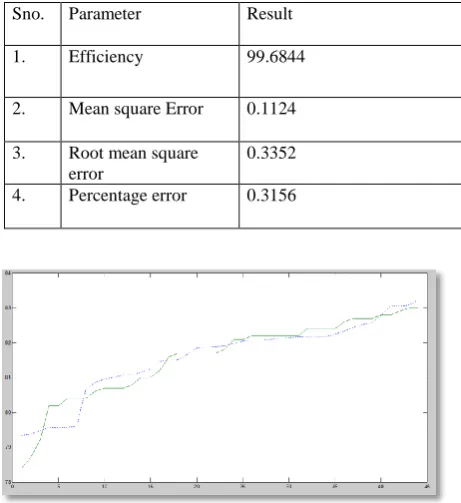
Sno. Parameter Result
1. Efficiency 99.6844
2. Mean square Error 0.1124
3. Root mean square error
0.3352
4. Percentage error 0.3156
Figure3.Plot between the noise observed and the noise obtained from the polynomial regression method of
prediction.
3.3 For K-nearest neighbour Algorithm
[image:4.595.315.544.452.716.2]In our scenario we have used k nearest neighbour algorithm to perform prediction on a certain test data by using training over certain another part of data, thus the data to be tested is checked for closeness with the data available in the training and if found significantly closed to the data in training then is provided with that particular information.
Table 2. For K-nearest neighbour Algorithm Sno. Parameter Result
1. Efficiency 99.7365
2. Mean square Error 0.1967
3. Root mean square error
0.4435
4. Percentage error 0.2635
3.4 For Artificial Neural Networks
The network training is carried out using Levenberg-Marquardt back propagation algorithm, and cross validation approach is used to perform the operation. The data set is divided into three main parts the first part is for the training operation while another part i.e validation is to tell when the neural network has been trained to the desired level of accuracy while the third part is the testing which is the data set which is to be tested.
The error of the training set gets smaller as the size of the tree grows. The idea of cross validation is to choose the representation in which the error of the validation set is a minimum. In these cases, learning can continue until the error of the validation set starts to increase.
[image:5.595.54.292.291.578.2]The validation set that is used as part of training is not the same as the test set. The test set is used to evaluate how well the learning algorithm works as a whole.
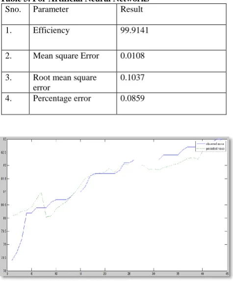
Table 3. For Artificial Neural Networks
Sno. Parameter Result
1. Efficiency 99.9141
2. Mean square Error 0.0108
3. Root mean square error
0.1037
4. Percentage error 0.0859
Figure5. Plot of predicted and the observed noise using neural networks back propagation algorithm
4.
CONCLUSION
This paper is an attempt to perform the prediction of noise levels which could be used in deducting the trends of noise and make further analysis about the creation of new highways, flyovers to reduce the road traffic concentration within a certain area and also to take steps forward in order to prevent the menace caused by the noise. After performing the analysis we found that Artificial neural networks give better results than any other prediction algorithm. The reason of preferring the neural networks over other algorithms are shown within the results. Multi linear regression and polynomial regression try to put on the data within a certain specified function which results in poor results compared to supervised learning. K-nearest neighbour algorithm however, giving better efficiency
then neural networks is more susceptible to over fitting then neural networks when the database is modified. Moreover, the data of the noise is generally noisy the neural networks are found to be having more capability of tolerating noisy data as well as they can classify on the patterns in which they have not been trained. Thus, providing better efficiency than any other algorithms in such kind of databases.
5.
FUTURE WORKS
The results of the prediction can further be used to identify the National Highways which are either most polluted or will be polluted in near future and then plan strategies to control it by either routing the traffic to through appropriate routes or other means.
6.
REFERENCES
[1] K. Kumar, V. K. Katiyar, M. Parida, and K. Rawat, ―Mathematical modelling of road traffic noise prediction‖‖, Int. J. of Appl. Math and Mech. pp: 21-28, 2011.
[2] K. Rawat, V. K. Katiyar, Pratibha, ―Mathematical Modeling of Environmental Noise Impact‖
[3] Kranti KUMAR, Manoranjan PARIDA and Vinod K. KATIYAR, ―Road Traffic Noise Prediction with Neural Networks-A Review‖, An International Journal of Optimization and Control: Theories & Applications, Vol.2, No.1, pp.29-37 (2012)
[4] V. Tripathi, A. Mittal and P. Ruwali ―Efficient Road Traffic Noise Model for Generating Noise Levels in Indian Scenario‖ International Journal of Computer Applications (0975 – 8887) Volume 38– No.4, January 2012
[5] Daniel, G.N, ―Cause and Effects of Noise Pollution.Interdisciplinary Minor in Global Sustainability‖, 1998.
[6] Fyhri, A. and Klæboe.R., ―Road traffic noise, sensitivity, annoyance and self-reported health —A structural equation model exercise‖ Environment International, v.35, pp: 91–97, 2009.
[7] R. Golmohammadi, M. Abbaspour, P. Nassiri, H. Mahjub ―A COMPACT MODEL FOR PREDICTING ROAD TRAFFIC NOISE‖, Iran. J. Environ. Health. Sci. Eng., 2009, Vol. 6, No. 3, pp. 181-186
[8] Prof. Thomas B. Fomby Department of Economics Southern Methodist University ―K-Nearest Neighbours Algorithm: Prediction and Classification‖
[9] Alfredo Calixto, Fabiano B. Diniz, Paulo H.T. Zannin ―The statistical modeling of road traffic noise in an urban setting Cities‖,Vol. 20, No. 1, p. 23–29, 2003
[10] S V Barai, A K Dikshit, Sameer Sharma Neural ―Network Models for Air Quality Prediction: A Comparative Study‖
[11]F. Sarmadian, R. Taghizadeh Mehrjardi and A. Akbarzadeh, ―Modeling of some soil properties using artificial neural network and multivariate regression in Gorgan province, north of Iran‖, Australian J. of Basic and Applied Sci., Vol. 3, No. 1, pp 323-329, 2009. [12]F. Karaca and B. Ozkaya, ―NN-LEAP: A neural
[13]F. Sarmadian, R. Taghizadeh Mehrjardi and A. Akbarzadeh, ―Modeling of some soil properties using artificial neural network and multivariate regression in Gorgan province, north of Iran‖, Australian J. of Basic and Applied Sci., Vol. 3, No. 1, pp 323-329, 2009. [14]R. K. Mishra, M. Parida, S. Rangnekar, ―Evaluation
and analysis of traffic noise along bus rapid transit
system corridor‖, Int. J. Environ. Sci. Tech., pp:737-750, Autumn 2010.
[15]Lars Kai Hansen and Peter Salamon ―Neural networks Ensembles‖ IEEE Tranasactions on pattern analysis and machine intelligence.Vol. 12, NO. 10, October 1990.