A generalised semi Markov reliability model

A generalised semi-Markov reliability model.

BENDELL, Anthony.

Available from Sheffield Hallam University Research Archive (SHURA) at:

http://shura.shu.ac.uk/19340/

This document is the author deposited version. You are advised to consult the

publisher's version if you wish to cite from it.

Published version

BENDELL, Anthony. (1982). A generalised semi-Markov reliability model. Doctoral,

Sheffield Hallam University (United Kingdom)..

Copyright and re-use policy

See

http://shura.shu.ac.uk/information.html

Sheffield Hallam University Research Archive

^ a O o

S h e ffie ld

City

Library

r e f e r e n c e

o n l y

Fines are charged at 50p per hour

2 6 MAR 2003

ProQuest Number: 10694221

All rights reserved

INFORMATION TO ALL USERS

The quality of this reproduction is dependent upon the quality of the copy submitted.

In the unlikely event that the author did not send a com plete manuscript and there are missing pages, these will be noted. Also, if material had to be removed,

a note will indicate the deletion.

uest

ProQuest 10694221

Published by ProQuest LLC(2017). Copyright of the Dissertation is held by the Author.

All rights reserved.

This work is protected against unauthorized copying under Title 17, United States C ode Microform Edition © ProQuest LLC.

ProQuest LLC.

789 East Eisenhower Parkway P.O. Box 1346

A GENERALISED SEMI-MARKOV RELIABILITY MODEL

by

Anthony Bendell B.Sc.(Econ), M.Sc., F.I.S., F.S.S., M.Sa.R.S.

Thesis submitted to the CNAA in partial fulfilment of the requirements for the degree of Doctor of Philosophy.

Sponsoring establishment: Collaborating establishment:

Sheffield City Polytechnic. National Centre of Systems Reliability, UKAEA.

\ j

« ( _{" \}

5l°l. 2.^7 ) I

_y

— Sc

-_ fr:o __

Anthony Bendell: A Generalised Semi-Markov Reliability Model

The thesis reviews the history and literature of reliability theory. The implicit assumptions of the basic reliability model are identified and their potential for generalisation investigated. A generalised model of reliability is constructed, in which components and systems can take any values in an ordered discrete or continuous state-space representing various levels of partial operation.

For the discrete state-space case, the enumeration of suitable system structure functions is discussed, and related to the problem posed by Dedekind in 1897 on the cardinality of the free distributive lattice. Some numerical enumerations are evaluated, and several recursive bounds are derived. In the special case of the usual dichotomic reliability model, a new upper bound is shown to be

superior to the best explicit and non-asymptotic upper bound previously derived. The relationship of structure functions to event networks is also examined. Some specific results for the state probabilities of components with small numbers of states are derived.

Discrete and continuous examples of the generalised model of reliability are investigated, and properties of the model are derived. Various forms of independence between components are shown to be

equivalent, but this equivalence does not completely generalise to the property of zero-covariance. Alternative forms of series and parallel connections are compared, together with the effects of replacement. Multiple time scales are incorporated into the formulation.

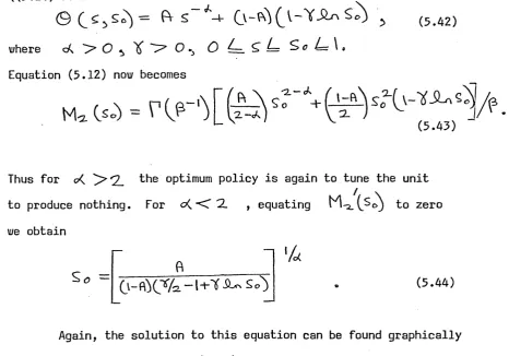
The above generalised reliability model is subsequently

specialised and extended so as to study the optimal tuning of partially operating components. Simple drift and catastrophic failure mechanisms are considered. Explicit and graphical solutions are derived, together with several bounds. The optimal retuning of such units is also

OBJECTIVES

The main objectives of the research in this thesis are:-(i) To investigate the nature of the basic reliability model,

to identify its implicit assumptions, and to examine their realism and potential for generalisation.

(ii) To construct a generalised model of reliability incorporating states of partial operation.

(iii) To consider the associated enumeration of such systems. (iv) To consider related optimisation problems in systems

management.

ADVANCED STUDIES

The following advanced studies were undertaken in connection with the programme of research for this thesis:

(i) Participation in research seminars at Sheffield City Polytechnic, Dundee College of Technology and the Universities of Sheffield and St. Andrews. (ii) Attendance at meetings/lectures of local groups of

the Royal Statistical Society, the Dundee Mathematical Association, and the Institute of Mathematics and its Applications.

(iii) Participation in the following conferences:

IMA Conference on the Mathematics and Statistics of Reliability, London 1975,

1st National Reliability Conference, Nottingham 1977,

11th European Meeting of Statisticians, Oslo 1978, 2nd National Reliability Conference, Birmingham 1979, 3rd National Reliability Conference, Birmingham 1981,

7th Advances in Reliability Technology Symposium, Bradford 1982,

EUROCON '82, Copenhagen 1982. (iv) Short secondments to:

The National Centre of Systems Reliability, during 1977, The Royal Military College of Science, during 1980.

(v) Appropriate reading.

During the registration period he has also acted as a referee for the IEEE Transactions on Reliability and the Journal of Physics Series A (Mathematical).

ACKNOWLEDGEMENTS AND INDIVIDUAL CONTRIBUTIONS TO JOINT RESEARCH Work for this thesis has been completed over a considerable period of part-time registration whilst the author was lecturing full-time at Sheffield City Polytechnic and subsequently Dundee

College of Technology. He would like to thank both of these institutions for their assistance and encouragement.

The thesis was originally conceived as concerned with the construction of a model for systems reliability at the level of greatest generality, with later chapters concerned with specific aspects of this generalisation. However, the breadth of this topic, together with the length of the period of registration and the

considerable amount of work published by the author in this area during this period, meant that the first draft of the thesis was long and unwieldy. In consequence, the thesis was redrafted to concentrate on the partial operation extension to the dichotomic reliability model, which formed Chapter 3 of the original version.

Though the general framework of the model and the treatment of each of the extensions to the usual dichotomic reliability

formulation was entirely the responsibility of the author, collaborative work took place with a number of colleagues on specific aspects of

was the major part of the identification, formulation and (where appropriate) analytic solution of the problems discussed. Numerical analysis, as well as the solution of illustrative examples, was largely done by the co-authors'.

The author would like to thank his collaborators on the above works, in particular Jake Ansell (now at the University of Keele) and Stephen Humble (now at the Royal Military College of Science) for their continued interest and perseverance in this collaboration. Thanks are also due to Colin Fraser (Dundee College of Technology) for his assistance with, and confirmation of, the evaluation of so many nasty integrals during the writing up of this thesis. He would also like to thank the staff of the National Centre of Systems

Reliability, and in particular Mr. A.J. Bourne, for useful discussion and assistance over a number of years. He is immensely grateful to his supervisors, Dr. M. Knott, Dr. W.G. Gilchrist and Dr. D.N. Shanbhag for their help and guidance, and for not giving up on him. Finally, the author would like to thank his wife, Sulli and Mary Combe for their help in the preparation and typing of this thesis, and the CNAA itself for having sufficient regulations to prevent him from avoiding to write up the thesis for any longer.

DECLARATION

CONTENTS

Pagg.

TITLE PAGE (i)

ABSTRACT (ii)

OBJECTIVES (iii)

ADVANCED STUDIES (iv)

ACKNOWLEDGEMENTS AND INDIVIDUAL CONTRIBUTIONS

TO JOINT RESEARCH (vi)

DECLARATION (viii)

CONTENTS (ix)

CHAPTER 1 INTRODUCTION

1.1 The Literature 1

1.2 Component Reliability 2

1.3 System Reliability 8

1.4 Possible Generalisations 25

CHAPTER 2

ENUMERATION OF MULTISTATE COHERENT SYSTEMS

2.1 Types of Multistate Coherent Systems 40

2.2 Terminology and Notation 43

2.3 Systems Enumeration _% 45

2.4 Bounds on the Number of Semi-Coherent Systems 48

2.5 The Special Case of

Q

2.6 Bounds in the General Case 51

2.7 Relationship of Event Networks to Structure

Functions 54

Page 59 61 63 66 77 82 95 106 110 114 125 133 138 142 147 150 153 CHAPTER 3

THREE AND FIVE STATE MODELS Introduction

Analysis of Three -State Models Analysis of Five-State Model

CHAPTER 4

A GENERAL PARTIAL OPERATION MODEL Formulation

Measures of Component Performance Component Independence

Series/Parallel Connections Replacement

Multiple Time Scales and a Random Environment CHAPTER 5

OPTIMAL TUNING

Introduction and Specialisation of Model Analysis of Catstrophic Failure

Page SUMMARY OF ADVANCES IN KNOWLEDGE ACHIEVED AND CONCLUSIONS

REFERENCES

APPENDIX

PUBLISHED PAPERS ON THE WORK OF THE THESIS*

A1 Generalisation of Dedekind's problem of the enumeration of coherent structures. (Proceedings of the Royal Society of Edinburgh, Series A, Vol. 89, 1981.) A2 Three-state and five-state reliability models

(IEEE Transactions on Reliability, Vol. R-29, 1980: Supplement, NAPS Document No. 03582-B, Microfiche Publications, NY).

A3 Operating history and failure and degradation tendencies. (IEEE Transactions on Reliability, Vol. R-27, 1978.)

Other papers by the author, published within the period of registration for Ph.D. but of more peripheral interest to the work of this thesis, appear in the reference list under his name or that of a co-author, as referenced in the text.

(xi)

CHAPTER 1 INTRODUCTION 1.1 The Literature

Whilst the exact age of Reliability Theory is subject to some dispute (e.g. Barlow and Proschan (1963), Lomnicki (1973)), there is general agreement that it has not yet celebrated its thirtieth birthday. Of the main reliability journals, the IEEE Transactions on Reliability first appeared in 1931, Technometrics in 1959, Microelectronics and Reliability in 1961, and Reliability Engineering in 1980. More recent journals also aim specifically to publish material on reliability, e.g. Stochastic Processes and Their Applications (since 1972) and the Journal of Statistical Planning and Inference (since 1977). Papers on reliability and related replacement problems are also more widely dispersed across the literature, and important in this context are Operational

Research Quarterly (1950-1977), Journal of the Operational Research Society (since 1978), Operations Research (since 1953), Naval

Research Logistics Quarterly (since 1954), and Management Science (since 1955). Microelectronics and Reliability incorporates the World Abstracts on Reliability.

The major reliability books started appearing in the 1960s with Bazovsky (1961), Lloyd and Lipow (1962), Cox (1962),

Zelen ed. (1963), Polovko (1964, English edition 1968),

Today regular symposia and conferences on reliability take place in the U.K., U.S.A. and elsewhere. The relevant organisations and professional bodies in the field, as well as the industrial history of reliability are reviewed by Green (1977). See also Brewer (1977).

The important early papers which established the basic characteristics of the reliability model and the problem of systems reliability predictions were von Neuman (1956), Moore and Shannon (1956) and Birnbaum, Esary and Saunders (1961).

1.2 Component Reliability

Reliability of a component of age t (t^O), denoted by R(t), is defined as the probability that the item is still operating satis­ factorily at that age, and R(t) is taken to be monotonically non-

increasing with R(0)=1, R(O O) = 0. Related functions to this reliability or survivor function are the distribution function of time to failure

F(t) = l-R(t),

(

.

)

its derivative the probability density function of time to failure (if it exists everywhere)

(

1

.

2

)

and the hazard function, age-specific failure rate or failure intensity

h(t) = f(t)/R(t). (1.3)

Clearly, R(t) f(t)

Also of interest is the cumulative hazard

(1.5) and the moments of the time to failure distribution (if they

exist), in particular the mean time to failure (MTTF)

i oo

A

CO

POU

E(t) = JJtf(t)dt = J 0R(t)dt «

(1.6)

It is common to restrict attention to specific classes of life or time to failure distributions defined in terms of the above functions. Of greatest practical interest are classes of distributions which in some sense correspond to \i/earout or aging. Barlow, Marshall and Proschan (1963) and Barlow and Proschan (1963) consider the class of distrubutions with increasing hazard or failure rate (IFR), for which h(t) is increasing in t. Birnbaum, Esary and Marshall (1966) consider the increasing failure rate average (IFRA) class for which H(t)/t is increasing. Bryson and Siddiqui (1969) consider the class with decreasing mean residual life (DMRL) for

f co

dt is decreasing. Marshall and Proschan (1963) LJoR(s+t)/R(s)

which

consider both the new better than used (NBU) class for which R(s+t)^ R(s)R(t), and the new better than used in expectation

nflO

A C©

(NBUE) class for which JgR(s+t)dt^R(s) JgR(t)dt. Haines and Singpurwalla (1974) introduce a further class with decreasing

percentile residual life (DPRL), whilst Muth (1980a) defines the class with convex decreasing mean residual life, which is a proper subset of the IFR class. See also Marshall and Proschan (1972), Esary, Marshall and Prosohan (1973), Proschan and Serfling (1974), Barlow and Proschan (1973), Hollander (1978) and Ross (1979). Tests of the appropriateness of the various classes are developed by Proschan and Pyke (1967), Barlow and Proschan (1969), Bickel and Doksom (1969), Bickel (1969), Hollander and Proschan (1972, 1974) and Koul (1977).

Multivariate equivalents have also been considered (e.g. Harris (1970),

Brindley and Thompson (1972), Marshall (1975), Buchanan and Singpurwalla (1977), Esary and Marshall (1979), Block and Savits (1980, 1981a)).

Whilst any continuous density on [o,eojmay be hypothesised for f(t), interest in the reliability literature (and especially

amongst reliability engineers) has concentrated upon the one-parameter exponential density

f(t) = |j- exp(-t/0)

R(t) = exp(-t/0)

n (1.7)

h(t) =

j

E(t) =

0,

02 , 0>O ,

since its constant hazard corresponds to random failure, or the central section of the so-called bath-tub curve popular amongst engineers (e.g. Shooman (1968), Lomnicki (1973)).

Despite e.g. Shooman (1968)'s early warning, it is still apparently true that many reliability engineers assume a constant hazard or age-specific failure rate unless there is evidence to the contrary (see e.g. Bourne (1973), Lomnicki (19.73), Cottrell (1977), Dorey (1979)), and this often causes serious error (Yasuda (1977), Moss (1978)). Indeed, in the literature reliability data is often presented implicitly based upon this assumption (e.g. Kujawski and Rypka

(1978), Gibson (1979), Snaith (1979), Henley and Kumamoto (1981)), and the administration of reliability data banks often shares this approach (e.g. George (1978), Silberberg (1979), Holmberg and Markling (1980), Colombo and Jaarsma (1980)). See also Shooman (1968)'s

comments on MIL-HDBK-217 and other published reliability data sources, and more recently Gaertner et al (1977), and O'Connor (1977).

a Markov Process, in this case a simple Poisson process, for the component (e.g. Feller (1968J. If upon failure the component is repaired and has an independent exponential repair time distribution,

Markov process. Some justification for the use of the exponential in systems is its arising as a limit* e.g. Feller (1971), Gnedenko, Belyayev and Solovyev (1970) . See also Gaver (1963), and SchOeller and Schwarz (1976).

the literature is the Weibull distribution named after Weibull (1939, 1951) but originally derived by Fisher and Tippett (1928). For this

The hazard function is monotonically increasing in t if p > l

(corresponding to aging, wearout or the third section of the bath-tub

to initial or burn-in failures, or the first section of the bath-tub). If j3= 1, the distribution reduces to the exponential (1.7).

model any section of the bath-tub curve partially explain the Weibull*s popularity in reliability work, as does its relationship to extreme value theory (e.g. Mann (1968)). One of its disadvantages is that standard methods of estimation are inconvenient; maximum likelihood estimation for example requiring iterative solution (e.g. Cohen (1965), Harter and Moore (1965, 1967), Wingo (1972), Ringer and Sprinkle (1972),

the alternating renewal process so generated forms a simple two-state

The other distributional form given increasing prominence in

0> 0, p>0.

curve), whilst it is monotonically (corresponding

Rockette, Antle and Klimko (1974), Zanakis (1979a), Archer (1980)).

However,alternative explicit estimation methods are available; Mann (1968) and Mann, Schafer and Singpurwalla (1974) give

extensive bibliographies. See also Hinds, Newton and Jardine (1977), Gross and Lurie (1977), Saylor (1977), Bennett (1977), Martz and Lian (1977), Kuchii, Kaio and Osaki (1979). In particular simple graphical estimation methods exist (e.g. Kao (1959, 1960),

King (1971), Cran (1976), Kaio and Osaki (1980)) and the appropriate special graph papers are commercially available (e.g. Chartwell 6572-3). Another disadvantage of the Weibull, relative say to the Gamma, is the complexity of results in renewal theory to which it leads (e.g. Cox (1962), Smith and Leadbetter (1963), Lomnicki (1966), Kay (1973), Nakagawa and Yasui (1978)).

The exponential and Weibull distributions above are respectively one and two parameter distributions. The fit to data can often be

improved substantially by the addition of an additional threshold parameter o(>0, so that each t in the right hand sides of f(t), R(t) and h(t) in (1.7) and (1.8) is replaced by (t-o0. (See Bob

Moss's contribution to the discussion of Lomnicki (1973)). Estimation, however, is correspondingly more complicated; e.g. Wingo (1973), Mann, Schafer and Singpurwalla (1974), Lemon (1975), Zanakis (1977, 1979a,b), Lehtinen (1979), Archer (1980), Dyer and Keating (1980).

The analytic inconvenience of the Weibull distribution has meant that a number of authors have investigated whether one can work satisfactorily with methods based on another distribution, usually the exponential, when the Weibull distribution applies. Zelen and Dannemiller (1961), although misquoted by Mann, Schafer and

Singpurwalla (1974),considered the robustness of four widely used

acceptance sampling procedures based upon the one-parameter exponential when the time to failure distribution was really two-parameter Weibull with an increasing hazard rate but the same mean life. They found that procedures based upon the recommendations of Task Group Two in

A.G.R.E.E. (1957) were very sensitive to departures from exponentiality, and that consequently applying them to data from a Weibull distribution with increasing hazard rate might result in substantially increasing the probability of accepting components having poor mean times to

failure. Harter and Moore (1976) show by Monte Carlo that the exponential based sampling plans in MIL-STD-781B are not robust under departures

from exponentiality and further give simple modifications for use when the Weibull distribution is appropriate. Posten (1973), also

building on the work of Zelen and Dannemiller, investigates the robustness of exponential-based reliability (point) predictions for series

systems of up to 15 identical components when the Weibull distribution is valid. Powers and Posten (1975) extend this to parallel systems. These two papers provide ranges of in which the error in using the exponential procedure is within an acceptable limit. Generally

these ranges are broader for the smaller numbers of components considered. Hager, Bain and Antle (1971) also demonstrate the lack of robustness of'exponential-based reliability estimation. For a connected Ba>esian problem, see Higgins and Tsokos (1977).

distribution, and the reliability for large time t.

1.3 System Reliability

The early papers on reliability by von Neuman (1956), Moore and Shannon (1956), and Birnbaum, Esary and Saunders (1961)

established the mathematical basis for the evaluation of the reliability of complex systems of components from knowledge of component reliability, and for the construction of reliable systems from relatively unreliable components. A methodology for the

computation of systems reliability from component reliability is

necessary as in most cases data on the reliability of complete systems or subsystems is virtually non-existent (e.g. Bourne (1973), Green and Bourne (1972), Snaith (1979)), and the complexity of the system and its often high reliability precludes the estimation of systems reliability by life tests on identical systems on time and cost criteria (e.g. Lomnicki (1973)). This point is given emphasis by the steady increase in the reliability of many components and thus systems through time (e.g. Kooi (1967), Shooman (1968)).

Whilst for single components for which life testing would take prohibitively long, the solution is accelerated life testing (i.e. life testing at environments more severe than those at which the component is expected to operate), this possibility is not available for complex systems. Accelerated testing (e.g. Mann, Schafer and Singpurwalla (1974)) was originally devised to provide failed components to be analysed so as to improve design. However, there is no guarantee that the basic physical processes of failure

encountered under excessively severe environments should be common

/

with those which would be encountered under long term exposure to a normal environment. According to Cox (1972) this is likely to

happen only when there is a single predominant mode of failure,

but see Kimball (1980).

For accelerated testing to provide a measure of the

reliability of a component under normal usage it is necessary to have some connection between the component's reliability under a normal

environment and its reliability under the excessively severe environments. Such a connection is sometimes no more than a purely graphical technique, though other times it is analytic and based on a theoretical model

of the mechanisms of failure. In fact, no satisfactory simple

connections exist for most components, although some generalised models with a theoretical background such as the Arrhenuis equation, are of some value. Often it is required to investigate in detail the physical structure of the particular component, model the operation of failure mechanisms upon these components, and then employ these theoretical mathematical models to obtain the connection between reliability under normal and excessively severe conditions (Jacobi (1968)). For complex systems, however, the assumption that the physical processes of failure under accelerated and normal environments are common is unlikely to be valid, as e.g. there will not be a single predominant mode of failure, and any connection between reliability under the normal and accelerated environments is likely to be

prohibitively complex. (However, see Nelson (1975)). Mann, Schafer and Singpurwalla (1974) discuss additional problems of accelerated life tests.

or equivalently u/hich combinations of operating components result in system operation. With the basic binary definition of reliability introduced in Section 1.2 and the usual implicit assumptions of the basic systems reliability model (given below), there are a number of equivalent representations of this aspect of system structure.

These are notably the structure function or truth table, the

reliability, event or switching network, and the Boolean hindrance or admission functions. See e.g. Hohn (1962),Flegg (1971), Green and Bourne (1972), Lomnicki (1973), Evans (1976).

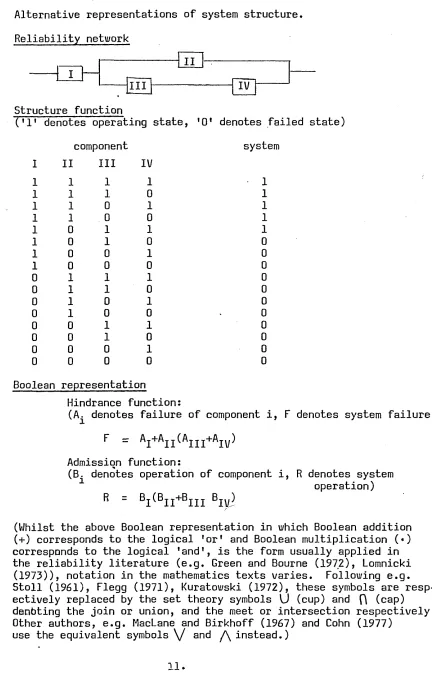
As an example of their application in the basic systems

reliability model, we show in Figure 1.1 these equivalent representations for a simple system which will only work if componentl and either II or (III and IV) work. An alternative representation which is not shown but which is gaining interest in the literature is event or fault trees (e.g. Barlow and Proschan (1975), Bazovsky (1977), Dhillon and Singh (1978)).

It is apparent from the figure that the implicit assumptions which make these representations equivalent - apart from the

assumptions that the system has a single function, the system's structure is static and components and system can each only take one

of two states - are that component and system operation is instantaneous, the order of component failures does not affect the state of the system, and that there is one unambiguous and homogeneous failure mode,

failure to operate (failure to idle is impossible). With these

assumptions, simple bounds of known accuracy can be put on the systems reliability for given component reliabilities by making use of the Inclusion-Exclusion Theorem and Bonferroni's Inequality (e.g.

Feller (1968), Lomnicki (1973)).

FIGURE 1.1

Alternative representations of system structure.

Reliability network

III Structure function

('l1 denotes operating state, '0' denotes failed state)

component system

II III IV

1 1 1

1 1 0

1 0 1

1 0 0

0 1 1

0 1 0

0 0 1

0 0 0

1 1 1

1 1 0

1 0 1

1 0 0

0 1 1

0 1 0

0 0 1

0 0 0

Boolean representation

Hindrance function:

(A^ denotes failure of component i, F denotes system failure)

F = Ai+Aii(Ai n +/W Admission function:

(B. denotes operation of component i, R denotes system operation) R = BjCBjj+Bjjj BivJ

(Whilst the above Boolean representation in which Boolean addition (+) corresponds to the logical 'or' and Boolean multiplication (•) corresponds to the logical 'and1, is the form usually applied in the reliability literature (e.g. Green and Bourne (1972), Lomnicki

(1973)), notation in the mathematics texts varies. Following e.g. Stoll (1961), Flegg (1971), Kuratowski (1972), these symbols are resp­ ectively replaced by the set theory symbols U (cup) and f\ (cap) denbting the join or union, and the meet or intersection respectively. Other authors, e.g. MacLane and Birkhoff (1967) and Cohn (1977)

To proceed further and be able to evaluate the reliability

function of the system (for any t) from the reliability of the

components it is necessary to have information or make assumptions

about the interrelationships of component failures, or equivalently

of the dependence between the states of the various components. The

basic system reliability formulation assumes that component

failures are independent, or equivalently the absence of common-mode

or common-cause failures, so that systems reliability can be obtained

from the usual rules for combining the .probabilities of independent

events (e.g. Birnbaum, Esary and Saunders (1961),Shooman (1968),

Bourne (1973), Lomnicki (1973), Edwards and Watson (1979)). With

this assumption, the reliability function for the system of Figure 1.1

is

R(t) = R1(t)jRlI(t)+RI1I(t)RIV(t)-Rn (t)R1II(t)RIV(t)l .

For complex systems, however, the computation of system's

reliability by such a direct method can be difficult even under

the assumption of independence, and methods for simplifying and

computerising evaluation are of practical interest to the reliability

assessor (e.g. Shooman (1968), Misra (1970), Woodcock (1971),

Green and Bourne (1972), Rosenthal (1973), Aggarwal, Misra and

Gupta (1973 a, b r c), Fussell (1975), Sharma (1976), Lin, Leon and

Hwang (1976), Blin et al (1977), Nakazawa (1977), Satyanarayana and

Prabhakar (1978), Arnborg (1978), Aggarwal and Rai (1978), Rai and

Aggarwal (1978), Gupta and Sharma (1978a), Gopal, Aggarwal and

Gupta (1978b), Locks (1978, 1979b), Singh (1979), Boffey and Waters

(1979), Laviron, Berard and Quenee (1979), Misra (1979), Easton

and Wong (1980)).

The structure function in Figure 1.1 illustrates the fact

that with the above assumptions (but not necessarily including

independence of component failures) corresponding to n distinct

components each of which may be in either of two states - operating

(1) or failed (0) - there are 2n states for the system corresponding

to all combinations of operating and failed components. To each of

these states of the system may be assigned one of the two levels

1 or 0, so that there are possible systems of n components.

Thus the number of possible systems gets large very fast; for two

components there are 16 possible systems, for three components

236, and for four components 65,536. In theory, the smaller is

the number of possible system structures the less information is

needed for, and the easier is the identification of, the appropriate

structure function and reliability function for a real physical

system. Consequently, there has been considerable interest in the

literature (e.g. Birnbaum, Esary and Saunders (1961), Esary

and Proschan (1963), Lomnicki (1972, 1973, 1977), Barlow and Proschan

(1975)) in restricting the class of possible structure functions to

a sub-set which corresponds to the systems with real physical

analogues.

The class of series-parallel systems discussed e.g. by

MacMahon (1892), Riordan and Shannon (1942), Knddel (1950),

Carlitz and Riordan (1956), Lomnicki (1972, 1977), is too

restrictive to represent all such realistic systems, and does not

contain all the real systems to be found in the reliability texts.

In particular it excludes the so-called k-out-of-n (or k-out-of-n:G)

systems (whereby the system operates if any k or more of its

components operate), which are examples of symmetric Boolean

functions (e.g. Flegg (1971)), and are of great physical interest

Ansell and Bendell (1982a)). Birnbaum in the discussion of

Lomnicki (1973) suggested a generalised class of realistic systems

which contains the series-parallel and k-out-of-n systems, and

which is based on replacing single modules in a simple system by

k-out-of-n structures of components.

The class of 'realistic* systems which has received most

attention in the reliability literature, however, is the class of

so-called coherent (or monotonic) systems introduced by Birnbaum,

Esary and Saunders (1961). This class contains the two-terminal

systems of Moore and Shannon (1936), as well as all series-parallel

and k-out-of-n systems. A coherent system is a system of components

such that the system's state does not deteriorate from 1 to 0 if

a failed component is replaced by an operating one, and does not

improve from 0 to 1 if an operating component is replaced by a

failed one, and operates if all its components operate and fails

if all its components fail. Formally, we describe the state of an

n-component system by the state vector

s = (s^, •••» sn) th

where s ^ the state of the component may be 1 (operating)

or 0 (failed), and the resulting state of the system (1 or 0) is

described by the structure function f(sO. Then if we define

1 = (1, 1, ..., 1)

£ = (

0

,

0

, ...,

0

)

and

if xdC^

~

and ^or some ^ >

it follows that a coherent system is defined by the requirements

f(x-)> f(j£) for all

x^> £

f(l) = 1

(

1

.

10

)

f(0) = 0 .

The definition of coherent systems in the literature vary

somewhat from the original one above due to Birnbaum, Esary and

Saunders (1961), although this is also used by some other authors,

e.g. Esary and Marshall (1974). Lomnicki (1973, 1977) neglects to

include the conditions (1.10) in his definition of coherent systems,

so that his 'coherent systems' correspond to semi-coherent systems

as defined by Birnbaum, Esary and Saunders (1961). However, this

is an omission rather than an alternative definition, since his

enumerations correspond to the original definition. Barlow and

Proschan (1965) refer to the coherent systems of Birnbaum, Esary and

Saunders (1961) as 'monotonic systems' due to the obvious algebraic

connotation. However, Barlow and Proschan (1975) perhaps following

Kaufmann (1969) re-define monotonic systems to be those satisfying

(1.9) alone; i.e. the semi-coherent systems of Birnbaum, Esary and

Saunders (1961). Their definition of coherent systems is composed

of the condition (1.9) together with the requirement that every

component is relevant; i.e. that there is no component c< for which

f (s i» •••> Soi-i»1,ik + i > * * * ’ s n^ =

f(si, •••» s* - l ’ °» s^ + l » •••» sn^

for all s ^ ... s^ , s^+1, ..., sn , (1.11)

It follows from tHis requirement of relevancy and from (1.9) that

(1.10) must also hold, but the definition is more restrictive than

the original one of Birnbaum, Esary and Saunders (1961). Phillips

(1977) uses monotonic in the same way as Barlow and Proschan (1965),

and coherent in the same way as Barlow and Proschan (1975). In this

thesis we shall follow the original definitions of coherency and

semi-coherency due to Birnbaum, Esary and Saunders (1961), except

Since coherent systems (by either the Birnbaum, Esary and

Saunders (1961) or the Barlow and Proschan (1975) definitions) are

generally regarded as corresponding to the set of real physical

systems of practical interest, a lot of attention in the literature

has been devoted to the study of the desirable properties possessed

by coherent systems. See for example Birnbaum, Esary and Saunders

(1961), Esary and Proschan (1963), Birnbaum, Esary and Marshall

(1966), Esary and Marshall (1974), Haines and Singpurvi/alla (1974), and

Barlow and Proschan (1975).

The reliability texts generally neglect to indicate that

the set of non-coherent systems does contain some very plausible and

indeed simple physical systems (see Evans (1978)'s review of Barlow

and Proschan (1975)), so that whilst coherency is to date the most

satisfactory criterion for systems to be of physical interest, it is

not completely satisfactory. It is perhaps interesting that when

John Bourne in the discussion of Lomnicki (1973) raised the question

of whether there may not be other classes of structures of more physical

importance than coherent systems, and whether Mr. Lomnicki has

established coherent systems by a personal examination or whether he

has seen ways of doing so automatically", no response was received.

However, Lapp and Powers (1977) do consider a non-coherent system

associated with a nitric acid cooling process, and this is subject

to further debate in the December 1977, April 1979 and June 1980

issues of the IEEE Transactions on Reliability. Locks (1979a)

provides an interesting discussion of aspects of this system.

Fussell (1975), Locks (1978) and Amendola and Contini (1980) discuss

the occurrence of non-coherent systems, and Worrell produced a

relevant computer program as long ago as 1961 (Bell Telephone

Laboratories (1961)). More recent programs and approaches that

can deal with non-coherent as well as coherent systems are described

by Bennetts (1975), Caldarola and Wickenhauser (1977), Kumamato and

Henley (1978) and Locks (1979c). See also Ogunbiyi and Henley (1981).

As an example of a simple non-coherent system, the system

represented in Figure 1.2 is composed of four springs designed to

keep a load in place. As is apparent from its structure function,

the system is non-coherent since failure (breakdown) of a single

spring causes system failure as the load is pulled to one side,

whilst failure of two opposite springs leaves the system operating

(although less stable in relation to outside disturbances).

Whilst the number of series-parallel systems of n

components is now known for both the cases where all components

are distinct and where some are identical (MacMahon (1892), Knddel

(1950), Carlitz and Riordan (1956), Lomnicki (1972)), similar

results are not available for the class of coherent systems, for

which the number of systems of distinct components is only known

explicitly up to n = 7. The enumeration problem for coherent

systems is in fact identical to the problem posed by Dedekind in

1897 on the cardinality of the free distributive lattice generated

by the symbols s^, ...,

s^.

Saunders (1961) definition (/} ) are given in column two of

Table 1.1, whilst the numbers corresponding to the more restrictive

definition of Barlow and Proschan (1975) (tn) are given in column

three. It is perhaps noteworthy that the plot of date of

publication against n = 4, 5, 6, 7 is approximately linear (especially

FIGURE 1.2

A non-coherent system.

Load C

Structure function

component system

A B

c D

1 1 1

1

1 1 0

0

1 0

1

0

1 0 0

1

0 1

1

0

0 1 0

0

0 0

1

0

0 0 0

0

0 1 1 1

0

0 1 1 0

0

0 1 0

1

0

0 1 0 o'

0

0 0

1 1

1

0 0

1 0

0

0 0 0

1

0

Kn ow n nu mb er s of c oh er en t sy st em s of n di st in ct c om po ne nt s, wi th fi rs t pu bl is he d so ur ce s. c

o ^ ->

•H

p--P p~

•H On

C i— 1

•H '—^

U-_{0 •H}

T3 _O

/— v •H

ia C p" E ON O i—1 v-x c CO c

JO 4J 1— 1 CM ON <P CM <p

o rH On VO rA

m rH CO O <P

o r' •»

f-t VO LA o

D_ CO o

p- <p

•D •*

C p-

p-CO CM

VO•*

o <P

1— 1 rH

p_{CO •*}

CO CM

P"

On /— s. *—■>

CO o LA

c rH <p <'— . VO

o N_■' ON vo ON

•H 1— 1 i— 1

•P ~o V-r ON '—*

•H c rH

C •H JO v_x JO

•H Ot o o

U- 0 p "O p

O X) 3 p 3

T> _o0 JO_{C_)} CO X 13 o rH

NO .

ON i

rH 1— 1 <0- CO VO ON CM VO

*_/ 1— 1 VO LA On

1— 1 LA fA On

rH C r*

CO _ P- CO O

CM <P

-p ) CO o

0 _p-•* _CM•*

E CO

D₀ vo

XI_{c I—1}

p

•H •*

CO CM

Church’s result for n = 5 was unduly delayed) and a simple

least-squares fit predicts 1990 approximately for the publication of the

number of coherent systems of eight distinct components!

Since the numbers of coherent systems is in general

unknown, the obtaining of sharp upperbounds (and to a lesser extent

lowerbounds) for these has long been of interest; Dedekind (1897),

Gilbert (1954), Korobkov (1963), Hansell (1966) (misquoted by

Lomnicki (1977)), Kleitman (1969), Hanish, Hilton and Hirsch (1969),

Alekseev (1973), Kleitman and Markowsky (1975), Korsunov (1977).

The sharpest explicit and non-asymptotic upperbound published to

date is due to Hansel (1966) who proved that

J ^ n ^ 3 Mn (1.12)

where M is the middle Binomial _n coefficient i.e.

n!

M = _n

(n/2)! (n/2)! 5 lf n even

n * t* 5 if n odd ([n+l]/2) i ( [n-lj/2)’

However, in Chapter 2 we derive improvements to this bound as

bi-products of the generalisation to multistate systems.

The above discussion is for the case where all the components

are distinct. Lomnicki (1977) discusses enumeration for the case

where some or all of the components are identical, and tabulates the

corresponding numbers of possible coherent systems (according to the

Barlow and Proschan definition) of up to five components. Coherent

systems with all the components identical have received some

attention in the reliability literature since they are of interest

in the context of the problem of optimal redundancy in the presence

of opposite failure modes (e.g. Lomnicki (1977), Phillips (1980),

Ansell and Bendell (1982a)). It is also true that for series-

parallel systems the enumeration problem was first solved for

identical components (MacMahon (1892)). For coherent systems,

making all the components identical also greatly reduces the numbers of

possible systems and consequently substantially simplifies (numerical)

enumeration. The available numbers of coherent systems of identical

components (due to Lomnicki (1977) are presented in column two of

Table 1.2

However, despite the earlier work of Phillips (1976) in a

related context, Lomnicki failed to consider the fact that a

further substantive reduction in the number of coherent systems

could be achieved by assuming independence of component failures

and considering the reliability function instead of the structure

function or Boolean function. With the usual assumption of independence,

systems with different Boolean or structure functions reduce to the

same reliability function. The corresponding reduced numbers of

distinct coherent systems up to n = 5 are shown in column three of

Table 1.2. As an example of the reduction, Figure 1.3 shows two

systems of four identical components with distinct Boolean representations

(even after rotation of the indices 1, 2, 3, 4) or equivalently

structure functions, but identical reliability functions under the

assumption of independence of component failures. (The reliability %

of each identical component is denoted by x). It follows from

Phillips (1980) that the reliability functions of coherent systems

of n identical components are, under the assumption of independence,

convex combinations of the reliability functions of the k-out-of-n

systems. Ansell and Bendell (1982a) generalise this result to

dependent components.

As a final point in this section, we note that Figure 1.3 serves

TABLE 1.2

Number of coherent systems of exactly n Identical components.

(Barlow and Proschan (1975)'s definition of coherency).

n distinct structure functions distinct reliability

Lomnicki (1977) functions

1 1 1

2 2 2

3 5 5

4 20 17

FIGURE 1.3

Two systems of identical components with distinct Boolean representations, but identical reliability functions.

(i)

Boolean function: ®l^2+ ^3^4

2 4

Reliability function: 2x - *

(ii)

or equivalently

Boolean function: ^1^2 +^2^3 +^1^3^4

model between event networks and Boolean and structure functions

(e.g. Flegg (1971)) can only be accomplished for non-series-parallel

systems by multiple representation of single components (which

reduces the event network to a formal statement of logical structure

without intuitive physical back-up), or by the multiple route notation

used in Figure 1.3 (which soon gets confusing as the numbers of

components and routes rise) or by ad-hoc logic devices such as the

k-out-of-n gate (e.g. Buzacott (1967,1970)) or the priority-AND

gate (e.g. Fussell, Aber and Rahl (1976)) which have become standard

notation in the engineering literature. The limitations of the

event network as a conveyor of system structure is a subject to

which we shall be returning when we consider the generalisation of

1.4 Possible Generalisations

The basic systems reliability model introduced in the previous

two sections is based on the following (often implicit) assumptions:

(i) Time t is continuous and perfectly ordered onQ),0^ .

(ii) The system has a single function (or output) which is

required to be performed continuously and does not vary

in time, and which depends for satisfactory operation

upon the operation of the components in the way specified

in the event network or structure function or alternative

representation of system structure.

(iii) The system’s structure, the environment of the system,

and the conditions that define component failure are

stationary in time.

(iv) Components and the system can each only be in one of

two homogeneous states at any point in time; 1 (operating)

or 0 (failed). At time zero they are in state 1.

(v) In the absence of a repair or replacement mechanism the

component state 0 is an absorbing state whilst the initial

state 1 is not, so that by time components and coherent

systems are in state 0, and the probability that any

component, or coherent system, is in state 1 is a

monotonically non-increasing function of time.

(vi) The operation of the components and system are

simultaneous and instantaneous.

(vii) The order of component failure does not affect the state

of the system for a given set of failed components.

(viii) The states of the components are independent.

specialisation, limit the application of the basic systems reliability

model. They are expressed as generally as is consistent with the

procedure for evaluating systems reliability introduced in the last

section. Whilst these assumptions form the norm in reliability work

(e.g. Barlow and Proschan (1965), Shooman (1968), Kaufmann (1969),

Lomnicki (1973)), they are often fully or partly implicit (especially

assumptions (i), (ii), (iii), (vi) and (vii)) and the situation is

further confused by the fact that in parts of the theoretical develop­

ment of reliability certain assumptions are unnecessary or can be

treated more generally. For example, the paper by Birnbaum, Esary

and Saunders (1966) avoids the element of time, and of the remaining

assumptions only makes explicit the assumptions that components

and systems only have t\i/o states and that the states of the components

are independent. For much of their development Barlow and Proschan

(1975) avoid the restrictive assumption of independence.

As one would expect from its wide-spread literature and use,

the basic systems reliability model corresponding to the above

assumptions fits reasonably well many real systems, or at least can

be regarded as a first approximation (e.g. Green (1977), Cannon and

Jones (1977), Snaith (1979)). Practical reliability engineers find

the complexity of reliability theory hard enough even in this

restricted form, without the complications of further mathematical

models (as the discussion of papers at the First National Reliability

Conference indicates; e.g. National Centre of Systems Reliability

(1978)). Further, limitations in the availability of data, and in

certain cases of appropriate statistical techniques, for even this

basic reliability model (e.g. Evans (1971, 1974), Konarski and Evert

(1975), Rosenthal (1975), Levine and Vesely (1977), Green (1977),

Shooman and Sinkar (1977), Anderson (1979), Dhillon (1979c), Haas and

Batt (1980)), imply that developing more sophisticated models may

not be worthwhile. Certainly in my experience of attempting to

obtain appropriate data for generalisations to the reliability model

I found that even with the assistance and data banks of the National

Centre of Systems Reliability I was only rarely able to find

appropriate data.

However, the unavailability of data etc. is a 'chicken-and-

egg1 argument, since it is not unreasonable to suppose that

appropriate data will by and large not be collected until there is a

purpose for it in terms of a method of analysis based on a generalised

reliability model. Indeed, apart from the hand of chance, problems

must be defined in appropriate generalised terms before appropriate

data can be collected to help solve them (Venton (1977)). (Maruvada,

Weise and Chamow (1978) discuss a related 'chicken-and-egg1 problem

whilst the comments of Evans (1977) on the gulf between the reliability

researcher and the reliability practitioner are also relevant).

Whilst the above arguments of the realism and good fit of

the basic system reliability model, the complexity of potential

generalisations and the unavailability of appropriate data for them,

may be taken to preclude the development of a generalised model of

reliability, the questions remain as to what would be the effects of

liberalising the assumptions, and whether a more general model of

reliability could be constructed without such restrictive assumptions.

Further, the reliability literature already contains many partial

extensions to the basic system reliability model, which are usually

in the form of generalisations of one specific aspect applied in the

IEEE Transactions on Reliability and Microelectronics and Reliability,

and specific cases are discussed as appropriate below. However, some

more systematic attempts at generalising the basic reliability model

are to be found in Green and Bourne (1972), Murchland (1975) and

Barlow and Proschan (1975). See also Papazoglou and Gyftopoulos

(1977), Virtanen (1977), Singh (1978) and Garribba, Mussio and

Naldi (1980). The existence of such generalisations of the basic

systems model in the literature, although largely in a piecemeal

fashion, does suggest that there is a general feeling amongst

reliability workers that the basic model is inadequate to describe

many real physical systems, and a more general model is required.

(See e.g. Barlow, Fussell and Singpurwalla (1975) and the introduction

by the editors to Section 2 of Apostolakis, Garribba and Volta (1980)).

For reasons of brevity, this thesis concentrates on the

partial operation extension to assumption (iv), though one can easily

broaden the model to generalise the other assumptions. Of course,

there is much justification for the generalisation of a single

assumption at a time, since it clarifies the effect of that assumption

on the methodology and results, it prevents the development of a

prohibitively complex model with associated data and inferential

problems, and it fcorresponds to the situation in applications where

it is often the case that only one or two standard assumptions are

in question at any one time.

There has, in particular, been much recent interest in the

extension of assumption (iv) to incorporate multistate systems with

ordered states, in an attempt to describe partial or degraded

operation. A number of plausible extensions to assumption (iv)

authors (e.g. Murchland (1975), Caldarola and

Wickenhadser (1977), Papazoglou and Gyftopoulos (1977) and Singh

(1978))) work generally with multistate reliability models not

restricted to a single direct physical analogue for the set of

states, most either decompose the operating stage 1 (or equivalently

the failed state 0) into an ordered set of states representing

various degrees of partial operation or degradation (e.g. Lloyd and

Lipow (1962), Derman (1963), Mine and Kawai (1974a, 1975, 1977),

Proctor and Wang (1975), Singh (1976),Maruvada, Weise and Chamow

(1978), Thomas, Derbalian and Bischel (1980)), or decompose the failed

state 0 into states representing multiple failure modes.

That even the most simple equipment is often subject to a

•large number of distinct failure modes is well accepted in the

engineering literature, as is the necessity to often consider various •

modes separately due to their differing system implications in terms

of repair time, safety, etc.; e.g. B^e (1974), Pau (1974), Mann,

Schafer and Singpurwalla (1974), Hyun (M.Gen)(1975), Banfi, Garribba,

Mussio, Naldi and Volta (1976), Dhillon (1976a,b,c,1977c,1978d),

Proctor and Singh (1976a,b), McCool (1976), Barbour (1977), Dahiya

(1977), Thomas (1977), Gopal, Aggarwal and Gupta (1978a), Legg (1978),

Caldarola (1980a)*. But see also Codier (1968) and Fertig and Murthy

(1978). Elsayed and Ziebib (1979) solve the general N-failure-mode

Markov model, whilst Yamashiro (1980) extends the solution to general

repair time distributions, and Yamashiro (1982) introduces standby

units. Another extension using a mixture model is given by Muth (1980b).

Mine and Nakagawa (1978) also employ a mixture formulation3whilst

Annello (1968) discusses competing risks. Bendell and Samson (1981)

modes. Shooman (1968) classifies the failure modes according to

the three regions of the bath-tub curve, and Gorg and Kumar (1977)

classify them into various minor and major failures. The occurrence

of distinct failure modes has been reported in amongst other systems

marine equipment (Bjrfe (1974)), weapon systems (Gower (1975)),

nuclear systems (Proctor and Singh (1976a), Dhillon (1976a)),

mechanical systems (Martin (1980)), power transmission systems,

electrical systems and aerospace equipment (Dhillon (1977c)).

An important special case of the multiple-failure-modes

extension to the basic reliability model is the case of opposite

failure modes for systems which are required to operate at certain

times and idle at others (in violation of assumption (ii)).

Codier (1968), Allen and De Oliveira (1977), Fertig and Murthy (1978),

and Gopal, Aggarwal and Gupta (1978a) give some justification for

grouping diverse failure modes into such opposite categories. There

are many real systems for which such switching between the operating

and idling states is necessary or desirable e.g. electronic equipment

(Elburn and Knight (1975)), electrical distribution networks (Allen

and De Oliveira (1977)), protective systems (Choy and Mazumdar (1975),

Gibson and Knowles (1977), Kontoleon (1978b)), weapons systems and

other emergency equipment (Nakagawa (1978)), nuclear power plants

(Apostolakis and Bansal (1977)), computer hardware (e.g. Lewis (1964),

Tasun (1977)), inertial navigation and ships power control systems

(Kujawski and Rypka (1978)), and avionic equipment (Kern (1978)).

See also Weiss (1961), Gaver (1964), Srinivasan (1966), Ueda (1972),

Osaki (1972), Rdde (1974), Nakagawa (1974, 1977), Kapur and Kapoor

(1975, 1978a,b), Nakagawa, Sawa and Suzuki (1976), Sasaki and

Hiramatsu (1976), Sasaki and Yanai (1977), Srinivasan and Bhaskar (1979),

Singh, Aggarwal and Kulkami (1979), Sasaski and Yokota (1980),

Berg (1981).

The existence of opposite failure modes-failures to operate

and failures to idle (or 'open1 and 'short' or 'closed' failures,

or 'passive' and 'active' failures, or 'fail-to-safe' and 'fail-

to-danger') in such real systems is also well known. Green and

Bourne (1972), for example, tabulate the proportions of total

failures which are of each of the two types for common components such

as fixed resistors, capacitors, coils and pneumatic and hydraulic

components. Jordan (1978) considers an opposite failure mode model

for iso-isolators. The literature discusses the design of systems

of components subject to opposite failure modes quite extensively,

having recently given particular emphasis to the identification of

optimum redundancy; e.g. Moore and Shannon (1956), Gordon (1957),

Barlow, Hunter and Proschan (1963), Barlow and Proschan (1965),

Lomnicki (1973, 1977), Phillips (1976, 1977, 1980), Proctor and

Proctor (1977), Kaufmann, Grouchko and Cruon (1977), Kontoleon (1978a),

Nakagawa and Hattori (1980), Ben Dov (1980),Bendell and Humble (1981)

and Ansell and Bendell (1982a).

Whilst components subject to opposite failure modes can be

considered to be 'in any one of four states at any t - failing to

operate, failing to idle, succeeding to operate, and succeeding to

idle - the literature usually combines the two success states into

a succeeding to operate or idle as required state, and thus produces

a three-state representation, (e.g. Roberts (1964), Barlow and

Proschan (1965), Shooman (1968), Lomnicki (1973), Allen and De Oliveira

(1977)). However, Mathur and De Sousa (1975) amongst others do obtain

of indeterminate failures, for u/hich it is not known whether they

are failures to operate or to idle. See also Tasun (1977) and

Dhillon (1977a). In contrast the four-state model of Berg (1981)

employs states of succeeding to operate, failing to operate and

being operational or failed when undemanded.

Three-state reliability models have appeared quite extensively

in the literature since they can be obtained from a number of

alternative extensions to the dichotomic reliability model as well

as that of opposite failure modes, and in each case represent the

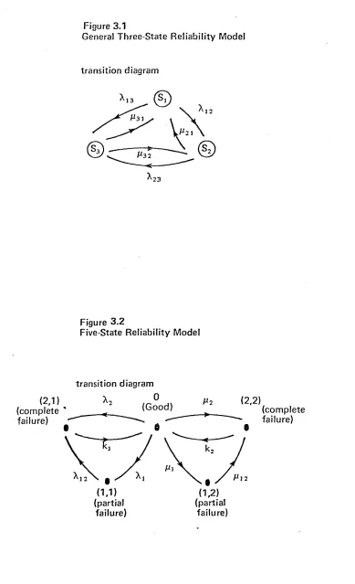
simplest such extension. The general three-state Markov model was

solved by Biggerstaff and Jackson (1969) in the context of power

generation in which the three states considered represented full

operation, derated operation and failure, so that the model

corresponds to the simplest partial operation extension to the basic

reliability model. The paper was subsequently overlooked in much of

the three-state literature since the papers of Kontoleon and Kontoleon

(1974) and Proctor and Singh (1976a) contain no more than the solutions

to the reduced versions of the general three-state Markov model

corresponding to the partial operation case with limited repair,

and the opposite failure mode case respectively. Proctor and Singh

(1975a) apparently independently re-solve the general three-state

Markov model, whilst Dhillon (1976a) does not even get as far as

deriving the explicit time dependent solutions of the opposite

failure mode sub-model (although in the context of complete/

catastrophic failures).

Endrenyi (1970), Endrenyi, Maenhaut and Payre (1973),

Grover and Billington (1974) and Allen and De Oliveira (1977)

in the context of electrical networks. See also Billington,

Allen and De Oliveira (1977). Regulinski (1980) also employs

a reduced form of the general three-state Markov model in studying

computer networks. See also Chan and Downs (1978) and Das, Hendry

and Hong (1980) for reduced forms of the three-state model in the

context of imperfect repair. Shenk (1977) considers the opposite

failure mode submodel (in the sense that two of the states are

not directly connected) but with the partial operation formulation.

The two repair time distributions are allowed to be Erlangian or mixtures

of exponentials. Kontoleon, Kontoleon and Chrysochoides (1975)

analyse throw-away maintenance for modules subject to both partial

and catastrophic failures, whilst Tumolillo (1974) has a three-state

random stress model. Braff (1977) uses a three-state Markov chain

model in which the states are operating, failed and pending failure

(which is assumed observable) to analyse the relationship between

failure rate and technician visitation. Phillips (1979) evaluates the

reliability and MTTF of a three-state system in which, apart from

full operation, the states correspond to the occurrence of revealed

and unrevealed faults. Mine and Kawai (1974b) consider preventative

replacement for a three-state unit with a wear-out state. Beichelt

and Fischer (1979,'1980) allow for two types of failure; those

removable by minimal repairs, and those needing complete replacement.

See also Mendenhall and Hader (1958), Cox (1959), Fischer (1977),

and Gorg and Kumar (1977).

Dhillon (1977c) discusses the steady state availability of

parallel (and series) systems of components subject to two failure

modes, whilst Singh and Proctor (1977) and Ksir (1979) consider

failure modes and/or partial failures. Dhillon, Sambhi and Khan

(1979) consider the analysis of a parallel network of components

subject to opposite failure modes and common-cause failures, whilst

Dhillon (1978c) consider a k-out-of-n system of three-state devices

also subject to opposite failure modes and common-cause failures.

Gupta and Sharma (1979) discuss a k-out-of-n system of three-state

units but with states of operating, failed and being installed,

whilst Dhillon (1979a) considers a four-unit redundant system with

common-cause failures and units subject to opposite failure modes,

and Chung (1979) extends this to an n-unit redundant system.

Dhillon (1979b) considers a complex system subject to partial

failures. Kumar andAggarwal (1978) analyse a two-unit warm standby

system with two types of failures, whilst Khalil (1977) and Singh,

Kapur and Kapoor (1979) consider a cold standby equivalent. See

also Elsayed (1979). Dhillon (1978d) considers a system of n standby

components subject to two failure modes. Takami, Inagaki, Sakino

and Inoue (1978) and Kumar and Kapoor (1979) discuss the employment

of fault detectors with opposite failure modes for series systems.

See also Inagaki (1980).

Butler (1979a) discusses importance measures and rankings for

three-state components in three-state systems, in which the states

correspond to the partial operation formulation. This is also

the case considered by Hatoyama (1979) who shows that the calculation

of systems reliability can sometimes be reduced to that of a

corresponding two-state system, and thus obtains methods of evaluation

and bounds for the reliability of three-state systems. He also

presents some reliability properties of systems with independent

components, and some bounds for systems with associated components.

Dhillon (1977b) provides a limited bibliography on three-state

models covering the period 1956 - 1976, whilst Virtanen (1977) gives

a partial review of three-state models up to 1975. See also

Sankaranarayanan and Usha (1980), Subramanian and Usha (1980), Locks

(1980), Lee (1980) and the nominally unrelated models of e.g.

Shooman (1968), Subramanian and Natarajan (1980), Allen and

Billington (1980).

Whilst the general three-state model and its sub-models

can thus have various plausible physical interpretations as extensions

to the basic dichotomic reliability model, the opposite failure mode

formulation does have the special feature that with it the expression

for a systems probability of failure to idle in terms of the

component probabilities of failing to idle (and failing to operate

if the system is non-coherent) can be obtained as the dual of the

expression for the systems probability of failing to operate in terms

of the components probabilities of failing to operate (and to idle).

See e.g. Lomnicki (1973). Thus apart from the study of specific

systems corresponding to specific opposite failure mode models which

were reviewed in the previous paragraphs^ and apart from the literature

on optimum redundancy for such components (reviewed previously), a

number of general' methodological papers appear in the literature on

the reliability analysis of systems of three-state components subject

to failures to operate and to idle; e.g. Proctor and Singh (1975b),

Singh and Proctor (1976), Gupta and Sharma (1978a), Gopal, Aggarwal

and Gupta (1978b), Nakagawa and Hattori (1980).

Just as it is possible to provide various physical inter­

pretations of three-state reliability models, it is equally possible