Data based Mechanistic Modelling (DBM) of Nonlinear Environmental Systems

M o d e l l i n g

(DBM)

o f N o n l i n e a r

E n v i r o n m e n t a l S y s t e m s

Christopher P. Fawcett, B.Sc. (Hons.)

A thesis submitted to the University o f Lancaster

fo r the degree o f D octor o f Philosophy

August 1999

Environmental Science Department

Institute o f Environmental and Natural Sciences

Lancaster University, United Kingdom

All rights reserved

INFORMATION TO ALL USERS

The qu ality of this repro d u ctio n is d e p e n d e n t upon the q u ality of the copy subm itted.

In the unlikely e v e n t that the a u th o r did not send a c o m p le te m anuscript and there are missing pages, these will be note d . Also, if m aterial had to be rem oved,

a n o te will in d ica te the deletion.

uest

ProQuest 11003635

Published by ProQuest LLC(2018). C op yrig ht of the Dissertation is held by the Author.

All rights reserved.

This work is protected against unauthorized copying under Title 17, United States C o d e M icroform Edition © ProQuest LLC.

ProQuest LLC.

789 East Eisenhower Parkway P.O. Box 1346

The experimental work described in this thesis was original work by the author

undertaken at the Department of Environmental Science, Lancaster University. The

material has not been submitted, in whole or in part for any degree, to this or any other

institution.

E

S

.

Submitted by

Christopher P. Fawcett, B.Sc. (Hons.).

A thesis submitted to the University of Lancaster

for the degree of Doctor of Philosophy

August 1999.

A

The main focus of the research studies presented in this thesis centre on the

application and development of data-based mechanistic (DBM) transfer function

models for nonlinear environmental systems. The data-based mechanistic modelling

approach exploits the available time series data, in statistical terms, to expose the

model structure, generating dynamic stochastic models that are parsimonious in nature

and can be interpreted in a physical manner.

For nonlinear systems, the DBM approach centres on the use of transfer function

models whose parameters are free to vary over time. The presence of such time

variable parameters may reflect either nonstationarity or nonlinearity; the latter arising

if the variations are also shown to be state dependent. Statistical time series methods

for estimating time varying parameters (TVP) and the use of these methods in state

dependent parameter modelling (SDPM) are discussed and applied to the modelling of

to investigate model uncertainty and over-parameterisation, set within the context of

data assimilation.

In each application, the DBM methodology is shown to successfully identify the

system nonlinearities, so providing additional physical insight and ensuring a good

explanation of the data with the minimum of model parameters (parsimony). Further,

the DBM approach provides an approach to both the evaluation and reduction in the

I would like to express my sincere gratitude to Professor Peter Young and Dr Arun

Chotai for their supervision and constant encouragement throughout the course of

these research studies. Dr John Rowan is also thanked for his guidance and

enthusiasm, and the assistance from Dr Mike Fasham is also appreciated.

Present and past members of the Systems and Control research group are also

mentioned for providing such welcome humorous relief from the computer terminals.

Paul deserves particular thanks for his helpful advice and suggestions. Mark, Glenda,

David, Simon and other colleagues from IENS are also thanked.

I am also grateful for the continued words of encouragement from friends and family

over the last four years. But most importantly, I would like to thank Laura for her

1. In t r o d u c t io n 1

1.1 Data-based mechanistic modelling 3

1.1.1 Transfer Function models 5

1.2 General scope of this thesis 9

1.3 Structure of this thesis. 10

2. Id e n t if ic a t io n a n de s t im a t io n o fl in e a r a n dn o n l in e a rs y s t e m s 13

2.1 General modelling procedure 14

2.2 General parameter estimation 15

2.3 Simplified refined instrumental variable estimation and model identification 17

2.3.1 Parameter estimation using the SRIV method 18

2.3.2 Model order identification 21

2.4 DBM identification and estimation of nonlinear systems 24

2.4.1 Background 26

2.4.2 Time varying parameter estimation using the Fixed Interval Smoothing 27

algorithm

Pass 1: ‘Forward Filtering’ 27

NVR estimation 30

Pass 2: ‘Backward Smoothing’ 31

2.4.3 State dependent parameter modelling 34

2.5 Stochastic and deterministic methods of parameter estimation 42

2.5.1 Deterministic parameter estimation: Nonlinear least squares 42

2.5.2 Stochastic parameter estimation: Maximum Likelihood 43

2.5.3 Linearised Kalman filter 45

2.5.4 ML estimation of continuous time nonlinear systems 48

2.5.5 Numerical optimisation algorithms 49

2.6 Conclusion 52

3. DBM

53

3.1 N icholson’s Lucila Cuprina experiments 53

3.2 M odelling N icholson’s blowfly 56

3.3 DBM modelling of Nicholson’s blowfly 60

3.3.1 Forward path linear TF model 61

3.3.2 TVP/SDPM Identification of the feedback nonlinearity 65

3.4 Optimisation of the deterministic blowfly model 70

3.5 Stochastic optimisation of the deterministic blowfly model 74

3.6 Extension of the stochastic blowfly model 79

3.7 Conclusion 87

4.

DBM

89

4.1 Rainfall-flow modelling 91

4.1.1 Unit hydrograph theory 91

4.1.2 Conceptual models 92

4.2 Transfer function rainfall-flow models 95

4.2.1 Lancaster DBM rainfall-flow model 96

4.2.2 IHACRES rainfall-flow model 100

4.3 Model calibration and validation 102

4.3.1 The data 102

4.3.2 Linear transfer function model 105

4.3.3 Lancaster DBM model results 106

4.3.4 IHACRES model results 112

4.3.5 M onte-Carlo analysis 114

4.4 Comparison of the measured soil moisture variables with generated 115

surrogate soil moisture series

4.4.1 Comparison of the measured soil moisture variables with the 116

Lancaster DBM soil moisture surrogate

4.4.2 Comparison of the measured soil moisture variables with the 123

IHACRES soil moisture surrogate

4.4.3 Data Series 2 126

4.4.4 Comparison between Data Series 1 and Data Series 2 126

4.4.5 Summary for nonlinear modelling of Data Series 1 and 2 128

4.5 Further TVP analysis 129

4.5.1 Model fits with sorted data 132

4.6 Lancaster DBM model modification 133

DBM

UK.

138

5.1 Wyresdale Park catchment and data 140

5.2 Rainfall flow model 144

5.2.1 Rainfall flow model on a seasonal scale 145

5.2.2 Rainfall-flow model for the 2 year time series 150

5.2.3 Rainfall-flow modelling and evapotranspiration 151

5.3 Suspended sediment load modelling 153

5.3.1 Wyresdale Rainfall-Sediment model 155

5.3.2 Wyresdale Rainfall-Sediment model for hindcasting 159

5.3.3 Reservoir sediment transmission model 161

5.4 Generating historical series 161

5.4.1 Monte Carlo uncertainty analysis 164

5.5 Validation of the model 165

5.5.1 Synthetic sediment accretion reconstruction 166

5.5.2 Lake sediment cores 167

5.5.3 Core extraction and analyses 168

5.5.4 Core validation 172

5.6 Concluding remarks 175

6.

178

6.1 Chapter aims and objectives 179

6.1.1 Data assimilation 180

6.2.2 M ixed layer dynamics 184

6.3 Three component NPZ ecosystem model 185

6.3.1 Simulink representation of the ecosystem model 189

6.3.2 Biological data 193

6.3.3 Data for parameters and calibration 196

6.4 Review of optimisation methods 196

6.5 Deterministic parameter optimisation 197

6.6 Model uncertainty and sensitivity analysis 205

6.6.1 Stochastic simulation modelling 207

6.6.2 Generalised sensitivity analysis 208

6.6.3 Uncertainty analysis of the TCE model using GSA 210

6.7 Parameter estimation by Maximum Likelihood 217

6.7.1 ML estimation results 218

6.8 Model linearisation and reduction 222

6.8.1 Classical linearisation and model order reduction 223

6.8.2 Data based approach to model order reduction and linearisation 224

6.8.3 Results of classical and DBM model linearisation 225

6.9 Conclusions 229

7. Co n c l u s io n sa n dr e c o m m e n d a t io n sf o rf u t u r er e s e a r c h 2 3 2

7.1 Data-based mechanistic modelling 232

7.2 Applications of DBM modelling 232

Figure 2.1 Figure 2.2 Figure 2.3 Figure 2.4 Figure 2.5 Figure 3.1 Figure 3.2

Figure 3.3

Figure 3.4

Figure 3.5

Figure 3.6

Figure 3.7

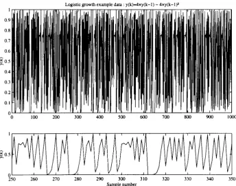
Response of the logistic growth equation 37

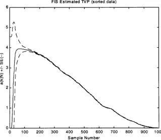
FIS estimate a{k I N ) with standard errors shown as a dashed 38

lines.

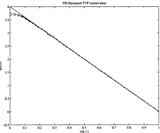
FIS estimate a{k I N ) versus y(k - 1 ) with standard errors 39

(red line). Actual nonlinear relationship 4 - 4 y ( k - \ ) (blue line).

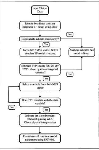
A summary of the complete DBM modelling procedure. 41

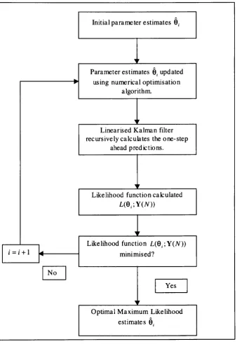
Summary of Maximum Likelihood procedure. 48

Numbers of blowfly Lucilia Cuprina in a population cage. 55

Linear transfer function model between eggs/day and blowflies: 63

Data (circles); Model (full line).

Model response to an impulse of 100 eggs (block) assuming 64

an initial blowfly population of 100 adults (full line).

FIS estimate of TVP from sorted data (full line) and standard 66

error bands (dashed line).

Estimated feedback nonlinearities: FIS non-parametric estimate 67

of u{k) versus y(k) (circles) with standard error bands

(dot-dashed); parameterised WLS estimate of non-parametric

result (dashed).

The optimised deterministic nonlinear model output (full line) 71

compared with the noisy measured data (circles).

Figure 3.8

Figure 3.9

Figure 3.10

Figure 3.11

Figure 3.12

Figure 3.13

Figure 3.14.

deterministic, optimised model output (full).

Model errors (top). The autocorrelation and partial 73

autocorrelation functions for the least squares optimised

model are shown in the bottom left and bottom right figures

respectively. An instance above the dashed line in these

figures, indicates the model errors are correlated.

(a) M L optimised stochastic one-step-ahead predictions 77

(fine line) versus measured blowfly data (circles).

(b) Prediction Errors.

One-step-ahead-prediction errors (top), autocorrelation 78

(bottom left) and partial autocorrelation (bottom right)

functions for the stochastic model optimised by maximum

likelihood.

(a) One-step-ahead predictions (fine line) from the final 81

optimised stochastic model and blowfly time series data (circles)

(b) One-step-ahead prediction error series.

The output of the deterministic component of the final 82

stochastic model. Simulated blowflies (fine line) and

data (circles), Simulated Eggs/Day (fine line) and data (circles).

Multi-step-ahead predictions (fine line), standard errors 84

(dashed line) and blowfly population data (circles).

Estimated feedback nonlinearities: Non-parametric FIS 85

estimate (circles)with standard error bands (dashed line),

Figure 4.1 Soil moisture probes in situ at the Erienbach catchment. 103

Figure 4.2 M easured variables Data Series 1. 104

Figure 4.3 Measured variables Data Series 2. 104

Figure 4.4 Best constant parameter linear TF model between rainfall 106

and flow.

Figure 4.5 FIS estimate of TVP b0( k\ N) and standard error bands 107

(shown dashed), Data Series 1.

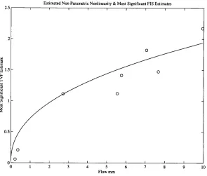
Figure 4.6 The most significant estimates of b0( k \ N) , shown as circles, 108

versus flow and the WLS estimate of the power law relationship.

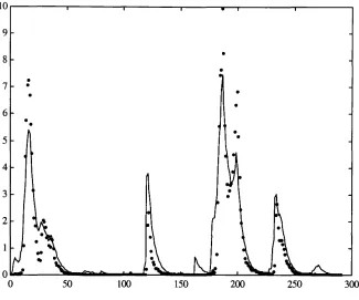
Figure 4.7 The [1,3,0] Lancaster DBM model (full line), [1,2,0] IHACRES 109

model (dashed line) and the observed data (dots).

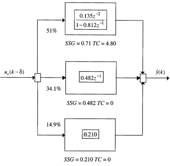
Figure 4.8 Parallel partitioning of flow processes. Where SSG denotes 111

the steady state gain and TC the time constant or residence time.

Figure 4.9 Parallel partitioning of the flow process. Where SSG denotes 113

the steady state gain and TC the time constant or residence time.

Figure 4.10 Parallel partitioning histogram. 114

Figure 4.11 (a) Surrogate soil moisture content lsm(k) (b) percentage 117

soil moisture content pwc(k) and (c) normalised inverse depth to

groundwater table,

Lancaster DBM model g w( k) , Data Series 1.

Figure 4.12 Simple regression of f ( k 1 N ) lsm(k) versus gw(k) 118

(a: Top Left b: Top Right) and soil moisture content p w c ( k)

(c: Bottom Left d: Bottom Right) from linear and non-linear

relationships, Lancaster DBM model, Data Series 1.

Figure 4.14 Estimates of (a: Top) Depth to groundwater table and 122

(b: bottom) soil moisture content from linear and nonlinear,

WLS relationships, Lancaster DBM model, Data Series 1. Data

(Dots); Linear relat. (Bold line); Nonlinear relat. (Fine line)

Figure 4.15 (a) Surrogate soil moisture content ihsm(k) , 123

(b) percentage soil moisture content pwc( k) , (c) normalised

inverse depth to groundwater table gw (k) , Data Series 1.

Figure 4.16 Estimates of depth to groundwater table and soil moisture 125

content from linear and non-linear, WLS relationships,

Lancaster DBM model, Data Series 1.

Figure 4.17 The most significant estimates of b0(k / N) versus flow and 130

the WLS estimate of two stage linear and nonlinear relationship,

Lancaster DBM model, Data Series 1

Figure 4.18 (a) Soil moisture surrogate lsm(k) , (b) percentage soil 133

moisture content pwc(k) and (c) normalised inverse depth to

groundwater table g w( k) .Lancaster DBM model, Data Series 1.

Figure 4.19 The most significant estimates of b0(k / N ) versus p w c ( k) and 134

the WLS estimate of the power law relationship.

measured data (dots).

Figure 5.1 Location map of Wyresdale catchment and reservoir. 142

Figure 5.2 Wyresdale Park catchment data. Rainfall measured at 144

Nicky Nook, flow and suspended sediment load measured at the

Wyresdale reservoir inflow, 15th May 1994 - 1st February 1996.

Figure 5.3 A section of the observed two year flow series (fine line) 151

and the nonlinear DBM model, (full line).

Figure 5.4 (a) SRIV estimated model residuals 15/05/1994 - 01/02/1996, 153

(b) Daily temperature (instantaneous measurement at 0900h),

measured at the Lancaster University Hazelrigg weather station

for the corresponding time period.

Figure 5.5 Schematic of the parameter optimisation procedure. 158

Figure 5.6 Nonlinear TF sediment model 159

Figure 5.7 Model fit of the hindcasting model 160

Figure 5.8 86 year (a)rainfall series (b)simulated flow, (c) simulated SSL 163

into the reservoir and (d) simulated SSL out of the reservoir

Figure 5.9 Cumulative sediment curves for the simulated 86 year SSL 165

output from the reservoir and the 2 year calibration data

Figure 5.10 Simulated sediment core (48cm deep in total): depth of 167

sediment deposited each year in millimetres (each successive year

1911-1995 is indicated by a different colour) reconstructed

deposition

Figure 5.12 Percentage content of sand, silt and clay in Core 2. 171

Figure 5.13 W et and dry bulk density of Core 2 172

Figure 5.14 Percentage sand content of Core 2 with dating chronology 173

Figure 5.15 Simulated and observed accretion sequence 174

Figure 6.1 Sim ulinkiconographic representation of the TCE Model 190

Figure 6.2 Sim ulinkiconographic representation of the Phytoplankton 190

System

Figure 6.3 Sim ulink iconographic representation of the Nutrient System 191

Figure 6.4 Sim ulink iconographic representation of the Zooplankton 191

System

Figure 6.5 Sim ulinkiconographic representation of the mixed layer 192

depth equations.

Figure 6.6 Sim ulink iconographic representation of the growth rate term. 192

Figure 6.7 Sim ulink iconographic representation of the mixing terms. 192

Figure 6.8 Repeated term. 193

Figure 6.9 Physical forcing terms of the ecosystem model 194

Figure 6.10 Observed nitrate, phytoplankton, NPP and zooplankton 195

concentration with ± one standard deviation uncertainty

Figure 6.11 Observation data (thin line) and simulation response to 200

optimised parameter set 1 (bold line) and 2 (dotted line ).

Units of concentrations are \lM N m3

Figure 6.12 Typical examples of a behavioural (dotted line) and non- 212

Figure 6.13

Figure 6.14

Figure 6.15

Figure 6.16

Figure 6.17

Significantly different B and B responses observed for 214

Parameter Set 1 parameter m.

Significantly similar B and B model responses observed for 214

parameter Set 2, parameter Kx.

Dissimilarity between B and B probabilistic histograms, 215

for parameter y 2 (Set 2).

Simulated and ML estimated model output 219

Table 3.1

Table 3.2

Table 4.1

Table 4.2

Table 4.3

Table 4.4

Table 5.1

Table 5.2

Best identified linear TF models listed in order of Rj 61

The sampling interval of the data is one day

Average blowfly population density deduced by Nicholson 86

(1954) and obtained from the stochastic DBM model

Best 5 DBM nonlinear TF models ordered in terms of YIC 108

Best five IHACRES nonlinear TF models ordered in terms 112

of YIC

Nonlinear Lancaster DBM models, Data Series 1. 135

Nonlinear Lancaster DBM models, Data Series 2. 135

Best identified nonlinear rainfall-flow models and the statistical 147

fitting criterion for each seasonal period

The performance of calibrated models (horizontal) simulated 149

using data from other seasonal periods (vertical). For example,

when the model, calibrated on the data of Summer 1995

( Rj - 0.819), is simulated using the Winter 1995 rainfall

data, the subsequent simulated flow series compares to the

(Matear, 1995)

Table 6.2 Optimal model parameters with standard errors given in 200

parenthesis.

Table 6.3 Correlation coefficients of the parameters in Set 1 203

Table 6.4 Re-optimisation of Solution 1 parameters. Parameters marked 204

with an asterix are held constant.

Table 6.5 Significant parameters of the TCE model determined by GSA. 213

Table 6.6 Parameters estimated using the ML method. 219

Table 6.7 Cross correlation matrix of ML estimated parameters 220

Table 6.8 Values of input variables for model linearisation and order 226

reduction

Table 6.9 Steady state conditions (SSC) calculated by continuous 226

sim ulation o f the TCE m odel and by constrained optim isation,

Ma tl a b/Sim ulink Trim function.

Table 6.10 Best linear TF models identified between input series M and 228

C

h a p t e r

1

I

n t r o d u c t io n

Mathematical modelling spans a wide range of philosophies and methodological

approaches. Models of environmental systems are predominantly deterministic in

nature which, in line with current paradigm, favours models that provide a physically

interpretable structure. An alternative systems approach, which has its origins in the

field of engineering and statistics, provides models that are developed directly from

time series data. Environmental modellers are beginning to embrace this data-based

modelling approach, realising the value of the enhanced statistical model estimation

tools and the parsimonious nature of data-based models.

Deterministic or mechanistic mathematical models are generally formulated to have a

structure that closely resembles the physical, chemical or biological reality of the

system as perceived by the modeller using classical dynamic conservation equations

(mass, energy and momentum) and are, therefore, heavily reductionist in nature. As a

consequence, these models are limited by the modeller’s experience and overall

understanding of the system and often become extremely complex and nonlinear as

that the modeller perceives in nature. Furthermore, as the parameters of deterministic

models often have a perceived physical interpretation, the feasibility, cost and time in

obtaining sufficiently informative data for their estimation, result in the models

becoming extremely difficult to validate.

Conversely, purely data-based (black box or time series) models are generated without

any prior assumptions regarding the systems internal behaviour. The m odel’s

structure is identified and parameters estimated objectively from observational time

series data using appropriate statistically-based methods. As such, data-based models

are simple in structure and parsimonious; characterised by only the number of

parameters that can be justified by the data. While such statistical models have the

advantage o f being data-based and stochastic, they are dependent upon the availability

and quality of data and are, consequently, often unsuitable for simulation purposes.

Furthermore, because they do not attempt to relate physically to the system they

surmise, many scientists consider the overall value of these types of model as low and

reject there utility on physical grounds.

The data-based mechanistic (DBM) modelling approach is a hybrid of these two

modelling extremes. Rejecting the deterministic-reductionist philosophy, DBM

models retain the statistical advantages and parsimony of the data-based modelling

approach but address the desire for a physical interpretation of the model. In the

majority of cases, the DBM methodology has been applied to linear systems, or where

nonlinear systems have been approximated by linear models. In the main, this has

been due to a restriction of computing capabilities, limiting the development of more

the DBM philosophy is invoked with a focus on the modelling of nonlinear systems

using techniques that have been developed more recently (Young, 1984; 1988; 1993)

and allow for the effective identification and estimation of nonlinear models.

This chapter introduces the DBM philosophy, with a particular emphasis placed on

nonlinear systems, and presents the novel contributions of this thesis, where the DBM

methodology and techniques are applied to model several different environmental

systems.

1.1 D

-

The data-based mechanistic (DBM) modelling methodology is designed to be as

objective as possible, exploiting the available time series in statistical terms to expose

the m odel’s structure, rather than being based on prior assumptions, in order to

generate dynamic stochastic models that are parsimonious in nature. DBM modelling

is based around the simple input-output transfer function (TF) model, originally

derived in the control engineering literature and later exploited in discrete-time terms

in the statistical literature by Box and Jenkins (1970). Here, the TF model structure is

identified and its parameters estimated directly from the data using statistical methods.

This allows for any uncertainty associated with both the model and the noisy data; and

it ensures that the DBM model reflects only the dominant modes of the system

behaviour.

For nonlinear systems, the DBM modelling approach is centred around the utilisation

estimated from the time series by a powerful recursive Fixed Interval Smoothing (FIS)

algorithm (see e.g. Young, 1984; 1993). In this setting, any parameters that exhibit

significant temporal variation over the observation interval will reflect either non-

stationarity in the system (i.e. its characteristics change over time) or a nonlinearity in

the system dynamics. The modelling proceeds to determine whether any identified

time varying parameter can be related to any states of the system, so allowing for its

direct parameterisation into the model. If the nonlinearity has been effectively

identified and parameterised by the ‘State Dependent Parameter M odel’ (SDPM), then

the resulting nonlinear TF model will usually have time invariant parameters. A final

prerequisite of the DBM philosophy requires that, in addition to explaining the data

well, the final identified DBM model is credible in physical terms; in other words, it is

only accepted as a truly useful model of the system if its structure and parameters can

be interpreted in a physical manner.

As the DBM methodology is truly generic in its approach, it has been utilised over a

wide range of disciplines over the last 10 years, including the fields of engineering,

economics, biology, and environmental science. As an example of the range of DBM

applications: Lees et a l (1994) developed an online DBM flood forecasting model,

which utilises recursive time varying parameter estimation, for the River Nith in

Dumfriesshire; while at the other extreme, Jarvis et al., (1998) employed the DBM

modelling approach to investigate the dynamic response of plant stomatal conductance

to the reduction in atmospheric humidity. However, most of these applications

consider linear or near-linear systems. In this thesis, the same approach is directed

1.1.1 Transfer function (TF) models

Over the past 30 years, the extensive development of digital computing has

increasingly encouraged the development of systems models and theories expressed in

discrete-time terms, as opposed to continuous-time theories which tended to be

associated with analogue computing. Discrete-time models are based upon sampled

data and are often presented in terms of either the forward shift, zl , or backward shift

z~l operators which are defined as,

where x ( k) is a signal at the kth sampling instant. The transfer function model, which

derives from the use of such operators, is simple but effective in its approach, relating

an input signal to an output signal which, in discrete-time, is normally assumed to be

sampled regularly at a sampling interval of At time units. The discrete-time transfer

function model of a single-input, single-output (SISO) system takes the form,

y ( k) = B— ^ u{k - A) (1.3) A ( C ‘ )

where u ( k) and y ( k) are the discretely sampled input and output signals,

respectively, at the kth sampling instant (e.g. values sampled after kAt time units).

Here, A (z_1) and B ( z~l ) are the polynomials in the z ~X operator, defined as follows.

z lx ( k) = x (k + i) (1.1)

A( z 1) = 1 + a xz x +--‘ + a nz n (1.4)

B ( z ~ ' ) = b0 +bxz ~ ' + - + bmz~m (1.5)

The integers n and m are the number of parameters in polynomials (1.4) and (1.5)

respectively. No prior assumptions are made about the nature of the TF, which may

be marginally stable, unstable or possess non-minimum phase characteristics. Any

pure time delay in the system, which often characterises environmental systems,

appears in equation (1.3) as the delay of A time intervals associated with the input

u{k - A ) .

In this linear model (1.3), two physically meaningful properties can be derived from

the transfer function model if its eigenvalues are real and the model is stable: the

steady state gain and time constant. The steady state gain, G, defines the relationship

between the equilibrium output value when a constant input is applied to the system.

G is calculated by setting the z 1 operator in equation (1.3) to unity such that, in the

case of a first order TF,

G = - ^ -

(1.6)

1 + fl]

As a result, the steady state gain can be used to determine whether there has been any

physical gains or losses to the system. The time constant or residence time Tc is the

time required for the system output to decay to e~x (-37% ) of its maximum value in

t =--- — (1.7) log, ( - a , )

W here the polynomials in equation (1.3) have multiple-order (e.g. third order), the TF

model can sometimes be unambiguously decomposed into lower order (e.g. first or

second order) TF elements connected in serial, parallel or feedback form. For

example, a second order transfer function ( m = 1 and n = 2 in (1.4) and (1.5)

respectively) can be represented by two first-order TF models connected either in

parallel or in feedback. As such, the decomposition of multi-order TF models can

sometimes reveal useful information about the system’s internal behaviour that would

otherwise remain unknown.

In its present form, the constant parameter TF model defined by equation (1.3) is

suitable for modelling linear systems. As discussed in detail in Chapter 2, equation

(1.3) can be conveniently redefined into an alternative time varying parameter (TVP)

or state dependent parameter TF form, suitable for modelling systems that are either

non-stationary or nonlinear.

The approach to identifying systems using time variable parameter estimation used in

this thesis has its origins in the early 1970’s (e.g. Beck and Young, 1976), where the

Extended Kalman Filter (EKF) was used to infer the structural nature of models for

biochemical oxygen demand and dissolved oxygen in rivers. Since then, the use of

the EKF in this role has been explored in detail by Beck in a number of papers and

chapters in books e.g. Beck, (1985); Beck, (1987); Kleissen et al., (1990); Chen and

philosophical sense, with the alternative approach used in this thesis, although the

methodology apart from the exploitation of recursive estimation, is quite different.

Equation (1.8) below presents the general form of the time varying parameter TF

model. The nonlinear relationship existing between the system input u ( k ) and output

y ( k) is reflected by the time varying nature of the parameters.

m = u( k ) = h ' ( k ) + b , ( k ) z - ' + - + bm( t ) z - u( k ) ( 1 8 )

A ( k , z ) 1 + a x(k)z +--- + an(k)z n

In the situation where the model parameters vary rapidly (i.e. at a rate consecutive

with the variations in the states of the system itself), the behaviour of the time varying

parameters of TF (1.8) may be characterised by potentially nonlinear functions of

related variables that are present within a suitably defined nonminimum state space

(NMSS) vector x ( k ) . The resulting general form of this state dependent parameter

TF model is defined as,

B { { x { k ) } , z ) y{k) =

A({*(*)},z )

= M x m + b 1{ % ( k ) ) z - ' + - + b j X ( k ) } z - m

l + allX(k))z-'+-- + aJXm z " ‘

where the NMSS vector x ( k ) is defined as,

(1.9)

X ( k ) = [y(/: -1 ), • • •, y(k - n)u{k)T, • • •, u(k - m)T U ( k ) T , - - , U ( k - q ) T J (1. 10)

and the terms b0\ x ( k ) } , bx{x(k)}, bm{x(k)}, ax\ x { k) } , an\ x ( k ) } indicate that the

vector of past values of the system output y ( k) ; present and past values of the

deterministic input variables u { k) that are considered to be the principle inputs to the

system; and vector the U ( k ) , which contains present and past values of additional

input variables that may affect the system nonlinearly. The thesis will argue that this

kind of ‘State Dependent Parameter M odel’ (SDPM) can provide a generic model for

the identification and estimation of a wide class of nonlinear systems within the

environmental and ecological sciences.

1.2 G

A summary of the overall aims of this thesis is given below.

□ This thesis emphasises the use of DBM methodology as a tool for modelling

nonlinear environmental systems. The techniques of time varying parameter

(TVP) estimation and state dependent parameter modelling (SDPM) which are

fundamental to objective nonlinear model development, are applied throughout

this thesis.

□ The DBM methodology is applied to environmental applications, specifically

modelling of nonlinear ecological and hydrological systems.

□ The DBM modelling philosophy generally rejects the use of large deterministic

models for systems where there is an abundant of quality observational data.

However, the use of much larger simulation models, which reflect the current

are available. But we believe that such simulation models must acknowledge

the uncertainty of the environmental system under consideration.

Consequentially, the third aim of this thesis is to show how stochastically

defined simulation models and data-based statistical methods can be used, in

combination, for the analysis of environmental systems that are poorly defined.

In this manner, it is possible to identify the strengths and limitations of the

simulation model, investigate alternative modelling approaches, and provide

more information about the system under consideration.

1.3 S

The present chapter has briefly introduced the DBM methodology which will be used

throughout this thesis in different modelling applications. Chapter 2 discusses the

main statistical methods for the identification and estimation of linear and nonlinear

discrete-time models that are used in these applications. In particular, the following

two algorithms are described in detail: the Simplified Refined Instrumental Variable

(SRIV) algorithm (Young, 1984); and the recursive Fixed Interval Smoothing (FIS)

algorithm for time varying parameter estimation (see e.g. Young, 1984). Furthermore,

deterministic and stochastic methods for optimising the parameters of the final

nonlinear model are introduced, including the M aximum Likelihood method (see e.g.

Harvey, 1989).

Chapter 3 describes how the DBM modelling methodology can be used to effectively

model the nonlinear behaviour of the population dynamics in the data series of the

In Chapter 4, the Lancaster DBM nonlinear rainfall-flow model (Young, 1993; Young

and Beven, 1994) which incorporates an effective rainfall term as a physical indicator

of catchment antecedent soil moisture conditions, is validated for the first time using

groundwater table and soil moisture measurements. A comparison between the

nonlinear components of the Lancaster DBM and IHACRES rainfall-flow models

(Jakeman et al., 1990a) is made, with reference to field data collected by ETH, Zurich.

These data justify the form of the nonlinear component in the Lancaster model, which

is identified using DBM techniques and provides an alternative form of the model

where such additional data are available.

Chapter 5 investigates how the DBM methodology has been be applied to the small

upland catchment of Wyresdale Park, Lancashire, in order to extend contemporary

time series of suspended sediment load. A discrete-time TF model for the rainfall-

sediment relationship is identified and estimated from 2 years of field data. This

model is used, together with historical rainfall series, to simulate suspended sediment

load series over the past 100 years in order to generate a synthetic sediment flood

sequence for the catchment reservoir.

Chapter 6 presents a critical evaluation of a deterministic oceanic ecosystem

simulation model with the overall aim of incorporating it into a data assimilation

(Robinson et al., 1999) framework. By considering the deterministic simulation

equations of the system in stochastic form, statistical methods of Monte Carlo

Simulation (MCS) (see e.g. Young et al., 1996) and Generalised Sensitivity Analysis

(GSA) (Spear and Homberger, 1980) are used to expose the poorly identifiable

combined statistical linearisation and model order reduction procedure, to determine

whether a reduced, low order, model can be identified, which accurately describes the

dynamics of the ecosystem.

The final chapter summaries the contributions of this thesis and suggests some

possibilities for future research on the development and use of DBM modelling

C

h a p t e r

2

I

d e n t i f i c a t i o n

a n d

E

s t im a t io n

o f

L

i n e a r

a n d

N

o n l in e a r

S

y s t e m s

Over the last five decades much research has concentrated on developing methods for

model identification and estimation of linear systems (see e.g. Jazwinski, 1970;

Young, 1984). In contrast, because of the more complex nature of nonlinear systems,

the associated techniques for system identification and estimation are in a relative

stage of infancy. The main focus of the research studies presented in this chapter,

centres on the development of data-based mechanistic (DBM) transfer function (TF)

models for nonlinear systems and introduces the mathematical time series methods

that have been utilised for their identification and estimation.

The first section of this chapter presents a brief overview of the general modelling

procedure for both linear and nonlinear systems. Section 2.2 introduces the general

concepts of parameter estimation. In Section 2.3 the Simplified Refined Instrumental

Variable (SRIV) algorithm for parameter estimation and model identification for

and estimating models for nonlinear systems, specifically focussing on the recursive

filtering and powerful Fixed Interval Smoothing (FIS) algorithms.

2.1 G

There are four main stages in the process towards generating a DBM model of a linear

or nonlinear environmental system. The first stage involves the collection of time

series data that are sufficiently dynamic to enable the environmental system under

consideration to be described by a TF model. For most environmental systems this

stage will require the main input and output variables of the system to be identified

and relevant monitoring equipment installed to record their behaviour. However,

where possible, it is often extremely beneficial to perform carefully planned

experiments, where the system input(s) are controlled, such that the system is

perturbed over its full dynamic range.

Having obtained sufficiently informative time series data from the system, a ‘suite’ of

model structures is selected from which the best model is chosen. The models may

be: deterministic or stochastic; have a linear or nonlinear structure; have constant or

time varying parameters; involve more than one input and output variable; and have

different orders. The perception and experience of the modeller will determine what

class of model is added to the ‘suite’ and will often involve additional detailed

analysis of the time series data.

Having determined the ‘suite’ of models, the parameters of each model must be

but perhaps the most well known is the least squares (LS) algorithm. LS forms the

basis of a number of derivative algorithms including weighted least squares (WLS),

extended least squares (ELS) and generalised least squares (GLS). The favoured

parameter estimation approaches adopted in the research reported in this thesis are the

Simplified Refined Instrumental Variable (SRIV) and the M aximum Likelihood (ML)

methods which are discussed in following sections of this chapter. Further details of

these and other techniques can be found in many texts on the subject, including

Jazwinski (1970), Young (1984), Ljung (1987), and Soderstrom and Stoica (1989).

Finally, each of the models are evaluated by objective statistical identification criteria,

in order to select the ‘best’ overall model. When making this choice, the intended

purpose of the model should not be disregarded. In some cases, the mechanistic

interpretation of the optimal model structure may challenge traditional perceptions of

the systems internal behaviour and require further investigation.

2.2 G

This section introduces the general methodology underlying TF model parameter

estimation. Most parameter estimation techniques are based upon the formulation of a

cost function from the TF model equations which, when minimised, provides the

optimal estimates of the model parameters. Consider the following generalised

discrete-time, linear, TF model of a single-input-single-output (SISO) system,

where y ( k ) and u ( k) are the system output and input respectively at the kth time

instant; 5 is the system pure time delay; and A(z_1) and B(z~l) are the TF

denominator and numerator polynomials respectively, defined as,

A (z_1) = l + alz~1 H— t-a z~n

1 " (2.2)

B ( z - l) = b0 +blz - l -h- + bmz - m

where z~l is the backward shift operator, that is z~'y(k) = y ( k - i ); and the integers n

and m are the number of parameters in the respective polynomials. By rearranging

equation (2.1) a simple cost function can be formulated from the difference between

the observed system and estimated model output, which is described as the response

error e ( k).

A j

e(fc) = y (* )~ . , u ( k -5) (2.3)

A(z"‘)

However, this cost function is limited by its nonlinear parameterisation which can only

be minimised by numerical methods (discussed in further detail in Section 2.5.5). An

alternative arrangement of (2.1) yields the equation error (2.4) which is linear about

its parameters and can be subsequently solved analytically, avoiding the necessity to

utilise numerical techniques.

e(k) = [yC/OAU'1) - B( z~‘ )u(k - 5)] (2.4)

A(z )

One possible method of obtaining the analytical solution to (2.4) is to utilise the

'normal equation o f linear least squares' (see e.g. Young, 1984 for its derivation)

The linear least squares algorithm provides good model parameter estimates,

providing measured system data without any stochastic noise disturbance is obtained.

However in practice, the observed data is usually corrupted by undesirable structured

‘coloured’ noise. The linear least squares algorithm acts to amplify the effects of the

noise during the estimation process, further contaminating the data sequence such that

parameter estimates are biased (Young, 1984). As a result, the presence of any noise

on the data will cause the parameter estimates to be asymptotically biased, and

statistically inconsistent regardless of the length of time series data utilised in the

procedure.

2.3 S

R

I

V

ESTIMATION AND MODEL IDENTIFICATION

To overcome this fundamental limitation of linear least squares estimation, a suite of

instrumental variable (IV) algorithms has been developed (see e.g. Young, 1984) that

provides consistent unbiased parameter estimates which require no a priori statistical

information regarding the noise sequence. The Simplified Refined Instrumental

Variable (SRIV) identification and estimation method is an extension of the original

IV estimation procedure which was first introduced by Young (1970) and a

simplification of the Refined Instrumental Variable (RIV) approach (see e.g. Young,

1976; Young and Jakeman, 1979; Young, 1984). It was shown (Young, 1985), that

under the assumption that the noise process is a serially uncorrelated series of white

noise with Gaussian distribution, that the complex RIV estimation algorithm could be

2.3.1 Parameter estimation using the SRIV method

The SRIV algorithm was first introduced in the discrete-time domain but has since

been extended for modelling systems using the delta operator (Young, 1991;

McKenna, 1998) and in the continuous-time domain (Young and Jakeman, 1980;

Foster, 1995; Price, 1999).

For the purposes of estimation, the stochastic TF model (2.1) can be conveniently

rewritten in alternative vector format,

)>(&) = z(*)Ta + riOt);

where r|(/fc) = A ( z ' , )e(k) and the vector z( k) and parameter vector a are defined in

the general case respectively as,

z(£) = [- yih - 1) - y( k - 2), y(k - n), u(k), u{k -1 ), • • •, u(k - m ) J (2.6)

a

with dimensions determined by the polynomials of (2.1).

Instrumental Variable (IV) estimation involves the introduction of an instrumental

variable (IV) vector \ { k ) defined as follows,

Here, the instrumental variable x ( k) , is defined as the 'noise free' estimate of the

system output jc(£) and is assumed to be serially uncorrelated with the noise process

r](&). It is generated from the j - h h iteration of the following ‘adaptive auxiliary

m odel’,

In contrast to the simple IV method (Young, 1984), in the case of SRIV estimation,

x ( k) and the associated variables are ‘pre-filtered’ utilising the y'-ith adaptive estimate

of the auxiliary model polynomial A ( z~l) , in the following manner,

The adaptive pre-filter F. acts to remove any undesirable high frequency components

from the input signal, which would otherwise reduce the efficiency of the estimation

results, whilst retaining those frequencies that are essential for system analysis.

For a given sample size N, the non-recursive optimal SRIV estimate a of the

parameter vector a is then obtained from the solution of the following SRIV

algorithm,

(2.9)

(2.10)

_ * = i

where,

z*(k) = [- y \ k - 1),- / ( k - 2),- • • y(k - n)*, u ( k f , u { k - \ ) r -,u ( k -m ) f (2.13)

x*(k) = [—jc*(A:-1),— x ( k - n ) , u*(k), u * ( k - l ) , - - - u * ( k - m ) J (2.14)

In the first instance, to initiate the algorithm the a priori estimate of the IV vector

x * ( k) can be obtained from the 'auxiliary model' using linear least squares parameter

estimates. This preliminary IV vector is subsequently inserted into the SRIV

algorithm to yield an initial estimate of the parameter vector a . The statistical

efficiency of a is further refined through subsequent iterations of this procedure,

where at each iteration, the parameters of the adaptive pre-filter and auxiliary model

are updated. It has been demonstrated, however (Young, 1976, 1985; Young and

Jakeman, 1979), that optimum SRIV parameter estimates can be obtained following

only three iteration steps.

Having determined the optimal parameter vector a from the final iteration step, the

SRIV algorithm also generates the inverse o f the instrumental product matrix (IPM)

P ( N) defined as,

-l

(2.15)

and the covariance matrix P * ( N),

P \ N ) = c ? P ( N ) (2.16)

P(AD =

k=N

X m * ( k ) T

k=

1

k = N

x ( k ) y ( k )

k = 1

where an estimate a 2 of the noise variance a 2 can be obtained from model residuals

e ( k) where

e( k) = y ( k ) - x ( k ) ; and a 2 = — ' S ' e ( k f (2.17)

N t?,

The covariance matrix P * ( N ) provides essential information regarding the level of

uncertainty associated with each parameter estimate. The leading diagonal elements

of the matrix distinguish the variance of each parameter estimate whilst a measure of

the parameter covariance is provided by the matrix off diagonal elements. In this

regard, the covariance matrix can be utilised within the context of Monte Carlo

uncertainty and sensitivity analyses (see Chapters 4 and 6).

2.3.2 Model Order Identification

Having estimated the parameters of a variety of different models, an optimal model

structure must be selected. Model order identification, namely the process of

identifying the most appropriate values of n, m and 5 in (2.1), is chiefly undertaken,

although not exclusively, with the assistance of carefully selected objective statistical

criteria. In combination, these objective methods should provide both a measure of

how well the model output explains the data and indicate the presence of model over-

parameterisation. In this study, model identification is based upon the coefficient of

determination, R j , and Young’s Identification Criterion, YIC, (see e.g. Young, 1989).

The coefficient of determination provides a statistical measure of how close the model

where a 2 is the sample variance of the model residuals e(k) (2.3), and a 2 is the

sample variance of the measured output y ( k) about its mean value y . Clearly, a

good model fit is obtained where the variance of the model residuals a 2 is low in

comparison to the variance of the data a 2 and the R 2 approaches unity. Conversely,

a poor model has a residual variance a 2 that is close to the magnitude of the sample

variance a 2 and the R 2 tends towards zero. It is important to differentiate R 2 from

the more conventionally adopted coefficient of determination R2. The latter is based

upon the variance of the one-step ahead prediction errors, rather than the model

response errors and, whilst this is a popular criterion for assessing the performance of

forecasting models, it is less suited for TF model order identification. In particular,

model one-step ahead prediction errors are relatively straightforward to minimise, as

the predictions are based upon past values of the system output itself; in contrast, the

model response errors are more difficult to minimise as the model output is

formulated based on the system input only. In a hydrological context, R 2 is also

commonly called the Nash and Sutcliffe efficiency criterion with unity power.

Although an excellent measure of model fit, the R 2 criterion should not generally be

utilised independently to assess the merits of a model, since it does not consider the

models relative complexity or the level of uncertainty associated with the parameter

For this reason, an additional statistical measure, which incorporates both of these

features, is utilised within the process of model identification. The heuristic Young’s

Identification Criterion Y IC, is defined as

rr2 1 i=np fT 2 f)

YIC = log, — + log, {ATEWV}; NEVN = — Y (2.19)

Gy np

,=1

where the variables of the leading term are defined as in equation (2.18);

np = n + m + 1 is the number of parameters in the TF model (2.1) denominator (n) and

numerator (m) polynomials; at is the ith element in the parameter vector a ( N ); p u is

the ith diagonal element of the covariance matrix P (A ) (where N is the total number

of samples); such that a p u is an estimate of the error variance associated with the ith

element of the parameter vector a ( N) after N samples.

The first term of equation (2.19) is a normalised measure of how well the model fits

the data; as the model fit improves, the ratio of decreases and the term

becomes more negative. The second term provides an indication of the relative

uncertainty of each ith parameter estimate, normalised with respect to all the

parameters in the npth order model; as the parameter error variance decreases, so the

parameter is better defined and the second term becomes smaller. A model that fits

the data well, but has a high order, with ill defined parameters, will have a

correspondingly high YIC value because of the large magnitude of the second term.

The YIC criterion, therefore, provides a compromise between model fit and over

parameterisation. An optimal model, with a low YIC, should give a good fit to the

In practice, the minimisation of the YIC will not necessarily identify the best overall

model and should, therefore, be used in conjunction with the R j criterion. This will

ensure that the model selected will fit the data well, without compromising parametric

efficiency and uncertainty. Additionally, it is important not to carry out the process of

model order identification without due regard to the physical nature of the system

under consideration. For example, if the system is known to have parallel or feedback

processes operating within it, model structures that can describe these behaviours

should be evaluated. Furthermore, the philosophy underpinning DBM modelling

should not be disregarded during the identification stage; a model structure that has a

clear physical interpretation may be favoured for selection over an alternative

structured model with slightly superior identification statistics. An additional, tertiary

model order identification criterion utilised in the research reported in this thesis was

the AIC criterion (see Box and Jenkins, 1970).

2 .4 D B M

IDENTIFICATION AND ESTIMATION OF NONLINEAR

SYSTEMS

Many environmental systems are non-stationary and nonlinear in nature and as a

consequence, alternative approaches to model identification and estimation need to be

adopted in order to develop models that successfully characterise their behaviour, e.g.

the EKF (Whitehead and Homberger, 1982; Chen and Beck, 1993). In this section a

novel DBM approach to modelling nonlinear systems is presented which has been

successfully applied in the areas of economics, ecology, biology, engineering and

1997; Young, 1998a). The DBM approach has the overall objective of identifying a

nonlinear TF with time invariant parameters through a process of objective statistical

inference applied to the time series data.

The preliminary stage of the DBM methodology is to determine that the system in

consideration is in fact nonlinear. This can be ascertained in the first instance, by

analysing the residuals of the best SRIV identified constant parameter linear TF

model, using standard statistical tests (e.g. Billings and Voon, 1986). In the second

instance, this may be achieved by allowing the parameters of a linear TF to vary over

time. The powerful Fixed Interval Smoothing (FIS) method of recursive estimation

(Young, 1993) can be used to obtain a non-parametric estimate of the model time

varying parameters (TVP). Any parameter that is found to be significantly time

variant over the observation interval, may reflect the non-stationary or nonlinear

behaviour of the system. Analysis then proceeds to investigate whether the identified

temporal parameter variations are state dependent and can be efficiently

parameterised. In accordance with DBM philosophy, in addition to enhancing the

model fit to the data, it is essential that the identified state has a clear mechanistic

interpretation in relation to the system under consideration. Having identified the

structure of the nonlinear dynamic model, the final stage of the DBM methodology is

to re-estimate all the model parameters against the time series through nonlinear

2.4.1 Background

The following discussion assumes that the behaviour of a discrete-time, dynamic

nonlinear and/or non-stationary environmental system can be represented by a general

dynamic, stochastic model which can be expressed as;

y(*) = 3 { x (* ),n (* )} (

2

20

where y ( k ) is the measured output of the system under consideration and 3{ } can be

regarded as a well behaved nonlinear function of the variables that are contained

within the non minimum state space (NMSS) state vector %{k) ,

X(k) = \y(k - 1), ■• ■■ ■■, y (k - n ) u ( k)T,■ ■■ •, u( k - m f V ( k f, • • • ,U (k - q)T f (2.21)

Here, %(k) constitutes a vector of past values of the system output y ( k) ; present and

past values of the deterministic input variables u{k) that are considered to be the

principle inputs to the system; and vector U ( k ) , which contains present and past

values of additional input variables that may affect the system nonlinearly, which at

this preliminary stage of the analysis, are yet to be determined. In addition, the

unobserved, serially uncorrelated, zero mean white noise process p(&), introduces the

stochasticity into the model and is assumed to be statistically independent to the input

variables u (k) and U ( k ) .

For explanatory purposes, consider a nonlinear system with only one principle input

reasonable to assume that the nonlinear model (2.20) can, in most cases, be

approximated by a linear TF with time varying parameters, which in the general form

can be written as,

y ( t ) = ^ ) + M * )z ' +’" ' ' +b" W z ” U(k) + S ( k ) (2.22)

1 + al (k)z +,-'-,+an(k)z

Here, the time variant nature of the parameters may reveal any non-stationary or

nonlinear behaviour present in the system. The noise term C,(k) arises from stochastic

disturbances in p ( £ ) .

2.4.2 Time varying parameter (TVP) estimation using the Fixed Interval

Smoothing (FIS) algorithm

Having presented the theoretical background to the DBM nonlinear modelling

concept, the following section discusses how the time variable parameters (TVP) are

estimated using a two pass recursive (forward filtering and backward smoothing)

operation on the time series data.

Pass 1: ‘Forward filtering’

In vector format, equation (2.22) can be represented in the form,

y (k) = z ( k ) Ta(.k) + r\(.k)Jc = 1,2 , - , N (2.23)

z ( k) = [- y(k - 1 ) ,- y(k - 2),— y(k - n)jt (k) ji( k — 1),- " u ( k - m j \ (2.24)

(2.25)

and where the noise process q(&) is assumed initially to be 'white' noise with variance

a 2. Having formulated model (2.21), it is necessary to characterise the temporal

variation shown by the parameters in vector a ( k) by some form of mathematical

description. One method, that has been demonstrated by Young (1978, 1984, 1993) as

capable of modelling these parameter variations, is the following Gauss-Markov

stochastic process,

where x(k) is a ‘state vector’ representing the parameters in a ( k) as well as other

elements that are necessary to characterise their complete temporal evolution. F ( k)

and G ( k) are transition and input matrices respectively and q{k) is a vector of

serially uncorrelated, random noise with zero mean and covariance Q. Here, the

transition matrix F { k ) determines the relationship between successive parameter

vectors, whilst the magnitude of parameter variation, introduced into the model by the

stochastic disturbance q ( k ), is regulated by the input matrix G ( k ) and Q. It is worth

noting, that when F ( k) and G{k) are both identity matrices, equation (2.24) can be

simplified to the well known random walk (RW) model,

x(k) = F(*)x(* -1 ) + G (*)q(*) (2.26)

It follows that from (2.26) that the best a priori estimate of vector x(fc), at the

previous time instant, is generated simply using,

x ( k \ k - l ) = F x ( k - l ) (2.28)

where the argument (k \ k - l) represents the estimate of x at time k, conditional on

the previous estimate at k-l. The a priori estimate of the covariance matrix associated

with equation (2.28) is obtained from,

V(k | k - 1) = F(k)P(k - 1)F(£)t + G0fc)QrG (* )T (2.29)

It has been shown (Young, 1984) that for estimation purposes, the ratio of Q and a 2

is important, rather than their explicit values. Therefore, the noise variance ratio

(NVR) matrix Qr is introduced into the estimation procedure and is defined as

Qr = Q / o l (2.30)

If model (2.23) was defined in its alternative state space form where the state vector

\ ( k ) = st(k) and the observation vector H(k) = z ( k)T , a recursive, prediction-

correction filtering algorithm for estimating the time varying parameters in model

(2.23) can be formed by combining equations (2.28 - 2.29) with a recursive time

variant form of the least squares parameter estimation algorithm. Thus, the ‘forward

pass’ of the TVP estimation routine is defined and takes the following form,

Prediction

x { k \ k - \ ) = ¥ { k ) x ( k - \ )