Assessing the Performance of a Prediction Error Criterion Model Selection Algorithm in the Context of ARCH Models

(1)

Munich Personal RePEc Archive

Assessing the Performance of a

Prediction Error Criterion Model

Selection Algorithm in the Context of

ARCH Models

Degiannakis, Stavros and Xekalaki, Evdokia

Department of Statistics, Athens University of Economics and

Business, Greece, Department of Statistics, University of California,

Berkeley CA, USA

2007

Online at

https://mpra.ub.uni-muenchen.de/96324/

(2)

A s s e s s i n g t h e P e r f o r m a n c e o f a P r e d i c t i o n E r r o r

C r i t e r i o n M o d e l S e l e c t i o n A l g o r i t h m i n t h e C o n t e x t

o f A R C H M o d e l s

Stavros Degiannakis

Department of Statistics, Athens University of Economics and Business, Greece

and

Department of Informatics and Biomedicine, University of Central Greece, Lamia GR-35

100, Greece

Evdokia Xekalaki

Department of Statistics, Athens University of Economics and Business, Greece

and

Department of Statistics, University of California, Berkeley CA, USA

Abstract

Autoregressive conditional heteroscedasticity (ARCH) models have successfully

been applied in order to predict asset return volatility. Predicting volatility is of great

importance in pricing financial derivatives, selecting portfolios, measuring and managing

investment risk more accurately. In this paper, a number of ARCH models are considered

in the framework of evaluating the performance of a method for model selection based on

a standardized prediction error criterion (SPEC).

According to this method, the ARCH model with the lowest sum of squared

standardized forecasting errors is selected for predicting future volatility. A number of

statistical criteria, that measure the distance between predicted and inter-day realized

volatility, are used to examine the performance of a model to predict future volatility, for

forecasting horizons ranging from one day to one hundred days ahead. The results reveal

that the SPEC model selection procedure has a satisfactory performance in picking that

model that generates “better” volatility predictions. A comparison of the SPEC algorithm with a set of other model evaluation criteria yields similar findings. It appears, therefore,

that it can be regarded as a tool in guiding one’s choice of the appropriate model for

predicting future volatility, with applications in evaluating portfolios, managing financial

risk and creating speculative strategies with options.

Keywords and Phrases: ARCH Models, Correlated Gamma Ratio Distribution,

Model Selection, Predictability, SPEC Algorithm, Volatility Forecasting.

1 . I n t r o d u c t i o n

To evaluate their accuracy, volatility forecasts have to be compared with realized

(3)

by Degiannakis and Xekalaki (2005) to indicate the ARCH model that generates “better”

volatility predictions, for a forecasting horizon ranging from one day to one hundred

trading days ahead.

Degiannakis and Xekalaki (2001) and Xekalaki and Degiannakis (2005) examined

the performance of the SPEC algorithm through the use of economic loss functions.

Degiannakis and Xekalaki (2001) made a comparative study among a set of ARCH model

selection algorithms in order to examine which method yields the highest profits by trading

straddles based on ten-days to forty-days-ahead variance forecasts. The results showed that

the SPEC algorithm achieved the highest rate of return. In the context of a simulated option

market, Xekalaki and Degiannakis (2005) have found that the SPEC algorithm performs

better than any other comparative method of model selection in forecasting one-day-ahead

conditional variance.

In this paper, we consider evaluating the SPEC method through the implementation

of statistical loss functions. Specifically, the performance of the SPEC algorithm is

examined through measuring the closeness of the volatility forecasts to the inter-day

realizations. The results show that the SPEC model selection procedure has a satisfactory

performance in selecting that ARCH model that tracks realized volatility closer, for a

forecasting horizon ranging from 16 days to 36 days ahead. So, it is possible to use this

model selection method in financial applications requiring volatility forecasts for a period

longer than one day, such as option pricing or risk management. The majority of studies

investigate the volatility forecasting accuracy for daily horizons, despite the fact that the

practitioners require predictions of lower frequency (the Basle Committee on Banking

Supervision (Basle Committee on Banking Supervision, 1998) for the use of Value-at-Risk

methods requires the estimation of 10-days-ahead volatility predictions, whereas fund

managers re-balance their portfolios on at least a monthly basis).

In section 2 of the paper, the ARCH process is presented. Section 3 describes the

SPEC model selection algorithm in the context of ARCH models. Section 4 provides a

brief description of the evaluation criteria and the inter-day realized volatility measures

considered. In section 5, the ability of the method proposed to select the ARCH model that

generates “better” predictions of the volatility, is examined. In section 6, the proposed model selection method is compared to other methods of model selection. Finally, in

section 7, a brief discussion on the results and on the merit of looking into the performance

(4)

2. T h e A R C H P r o c e s s

For Pt denoting the price of an asset at time t, let yt ln



Pt Pt1



denote the continuously compounded return series of interest. The return series is decomposed into

two parts, the predictable and unpredictable component:

 

tt t t E y

y  _|_₁  , _(2.1)

where E

 

yt|t1 is the conditional mean of return at period t depending upon the

information set available at time t1 and t is the prediction error. Usually, the

predictable component is either the overall mean or a first order autocorrelated process

(imposed by non-synchronous tradingi). The conditional mean, unfortunately, does not

have the ability to give useful predictions. That is why modern financial theory assumes

the asset returns are unpredictable. Before the start of the 1980’s, the view taken about

returns in financial markets was that they behave as random walks and the Brock et al.

(1987) [BDS] statistic has widely been used to test the null hypothesis that asset returns are

independently and identically distributed. This hypothesis, however, has been rejected in a

vast number of applications. A rejection of the null hypothesis is consistent with some

types of dependence in the data, which could result in from a linear stochastic system, a

nonlinear stochastic system, or a nonlinear deterministic system. Thus, a question arises:

“Are the nonlinearities connected with the conditional mean (so, as to be used to predict

future returns) or with higher order conditional moments?” Artificial neural networksii_, chaotic dynamical systemsiii, nonlinear parametric and nonparametric modelsiv are some

examples from the literature dealing with conditional mean predictions. ARCH modelsv

and stochastic volatility modelsvi are examples from the literature dealing with conditional

variance modeling. However, no nonlinear models that can significantly outperform even

the simplest linear model in out-of-sample forecasting seem to exist in the literature

(neither in the field of stochastic nonlinear models nor in the field of deterministic chaotic

systems). On the other hand, the ARCH processes and stochastic volatility models appear

to be more appropriate to interpret nonlinearities in financial systems on the basis of the

conditional variance. If an ARCH process is the true data generating mechanism, the

nonlinearities cannot be exploited to generate improved point predictions relative to a

linear model.

In the sequel, the conditional mean is considered as an th

order autoregressive

(5)

Assuming the unpredictable component in (2.1) is an ARCH process, it can be represented as:

 



, ,...; , ,...; , ,...



, 1 , 0 ~ 2 1 2 1 2 1 2         t t t t t t t iid t t t t g N z z          (2.3)

where

 

zt is a sequence of independently and identically distributed random variables, t

is a time-varying, positive measurable function of the information set at time t1, It1, t

is a vector of predetermined variables included in It and g



. could be a linear or

nonlinear functional form as is usually assumed in the ARCH literature. The unpredictable

component has variance 2

t

 , conditional on information given at time t1. The

conditional variance is a linear or nonlinear function of lagged conditional variances, past

prediction errors and predetermined variables measurable at time t1. The conditional

prediction error is normally distributed, but the unconditional prediction error and the

conditional variance of it have an unknown form of distribution. The conditional

standardized prediction error, zt|t1, is standard normally distributed:



0,



~

 

0,1

~ 1 1 | 1 | 2 1

|t N t ztt tt t N

t

  

    

 . (2.4)

In the recent literature, one can find a vast number of parametric specifications of

ARCH models motivated by the characteristics explored in financial markets. A

researcher, who is looking for the “best” model, would have in mind a variety of candidate models. The most commonly used conditional variance functions are the GARCH

(Bollerslev 1986), the Exponential GARCH, or EGARCH, (Nelson 1991) and the

Threshold GARCH, or TARCH, (Glosten et al. 1993) specifications. In the sequel, these

ARCH models are considered in the following forms:

The GARCH(p,q) model





_







       p i i t i q i i t i

t a a b

1 2

1 2 0

2  

 (2.5)

The EGARCH(p,q) model

 

_



 



       _                p i i t i q

i t i

i t i i t i t i

t a a b

1 2 1 0 2 ln ln        _(2.6)

The TARCH(p,q) model





_







          p i i t i t t q i i t i

t a a d b

1 2 1 2 1 1 2 0

2   

 , (2.7)

(6)

The majority of practical applications, i.e. option pricing, determination of the

value-at-risk, require more than one-day-ahead volatility forecasts. More than

one-step-ahead forecasts can be computed by repeated substitution. The forecast recursion relation

of the GARCH(p,q) model is:

 

_



 



_



 



        p i i t t i q i i t t i t t

t a a b

1 2 1 1 2 1 0 2 | 1

ˆ  

 (2.8.a)  

_



 



_



 



_



 



             p i s i t t i q s i for s i s i t t i q s i for i s i t t i t t s

t a a a b

1 2 2 1 2 0 2 |

ˆ   

 (2.8.b

)

For st, the forecast of the predictive error s conditional on information available at

time t equals to its zero expected value, E



s|It



0. On the other hand, the estimated

value of 2

s

 measured at time t should be equal to 2

|t

s

 for st. For st, the predictive

error and its square are computed by the model with the available information at time t.

The forecast recursion relationship associated with the EGARCH(p,q) model is:

 

_

   

_



 





                           p i i t t i q

i t i

i t t i i t i t t i t t

t a a b

1 2 1 1 1 1 1 1 0 2 | 1 ln ˆ ln       

 

_

   

_

 

_



 





                               p i s i t t i q s i for i t i q s i for s

i t i s

s i t t i s i t s i t t i t t s

t a a a b

1 2 1 0 2 | ln 2 ˆ ln         , (2.9.a) (2.9.b)

that associated with the TARCH(p,q) model is:

 

_



 



 

_



 



         p i i t t i t t t q i i t t i t t

t a a d b

1 2 1 2 1 2 1 0 2 | 1

ˆ    

  

_



 



_



 



 

_{ }

_



 



                   p i s i t t i t s t t q s i for i s i t t i q s i for i s i t t i t t s

t a a a E d b

1 2 2 1 1 2 1 2 0 2 |

ˆ     

 .

(2.10.a)

(2.10.b)

Here, E

 

dt denotes the percentage of negative innovations out of all innovations. Under

the assumption of normally distributed innovations, the expected number of negative

shocks is equal to the expected number of positive shocks, or E

 

dt 0.5.

The forecast of the conditional variance at time t over a horizon of N days ahead

is simply the average of the estimated future variance conditional on information given at

time t

 



    N i t i t N t N 1 2 | 1

2 ˆ

(7)

3. T h e S P E C M o d e l S e l e c t i o n M e t h o d

In this section, a brief description of the theoretical motivation of the SPEC

algorithm that is based on pairwise comparisons of the sums of squared standardized

one-step-ahead forecasting errors of a set of ARCH models is provided. Degiannakis and

Xekalaki (2005) introduced the SPEC model selection method based on the correlated

gamma ratio (CGR) distribution, which was derived by Xekalaki et al. (2003) as the

distribution of the ratio of two variables jointly distributed according to Kibble’s (1941) bivariate gamma distribution. Kibble (1941) proves that if, for t 1,2,..., the joint

distribution of



   B



t A t r

r , is the bivariate standard normal, then the joint distribution of

 



  T t A t r 1 2 1

2 and



 

  T t B t r 1 2 1

2 is Kibble’s bivariate gamma distribution. As pointed out by

Xekalaki et al. (2003),  A t

r and  B t

r could represent the standardized prediction errors

from two regression models (not necessarily nested) but with a common dependent

variable. The distribution of the ratio of the sum of their squares is the CGR distribution;

symbolically,     ~

 

,

1 2 1 2 k CGR r r T t A t T t B t



 

, where k T 2 and



   B



t A t r r Cor ,   .

Thus, two regression models can be compared through testing the null hypothesis of

equivalence of the models in their predictability against the alternative that model

 

A

produces “better” predictions. The null hypothesis is rejected if

   

_

_,__,_

_

1 2 1 2 k CGR r r T t A t T t B

t







 

, where CGR



k,,



is the 100



1



percentile of the

CGR distributionvii.

Degiannakis and Xekalaki (2005) assumed that we are interested in comparing the

predictive ability of two ARCH models:

Model A Model B

   

 



           



,... , , ,..., , ,..., 1 , 0 ~ 2 1 2 2 1 2 2 1 2 , 1 , 1 A t A t A q t A t A p t A t A t iid t A t t A t g N z z                     

 



           



,... , , ,..., , ,..., 1 , 0 ~ 2 1 2 2 1 2 2 1 2 , 2 , 2 B t B t B q t B t B p t B t B t iid t B t t B t g N z z                 

The joint distribution of



 



   

  



 

 _ T

t A t t A t t T t A t t z 1 2 1 | 2 1 | 1 1 2 1 |

1 ˆ ˆ

2

ˆ

2   and



 



   

  



 

 _ T

t B t t B t t T t B t t z 1 2 1 | 2 1 | 1 1 2 1 |

1 ˆ ˆ

2

ˆ

2  

is Kibble’s bivariate gamma distribution. Thus, the standardized one-step-ahead prediction errors can be used to test the null hypothesis of equivalence of the models in their

(8)

The null hypothesis is rejected if ˆ   ˆ  



,,



1 2

1 | 1

2 1

| z CGRk

z

T

t A t t T

t B t

t







   

. Note that the SPEC

algorithm is always computed on the basis of the one-step-ahead forecasts since zˆt1|t are

asymptotically normally distributed (Degiannakis and Xekalaki 2005), while the

standardized residuals from N-step ahead forecasts, zˆtN|t, for N 2, are not.

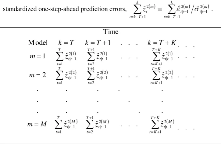
According to the SPEC model selection algorithm, the models that are considered

as having a “better” ability to predict future volatility of the dependent variable, are those

with the lowest sum of squared standardized one-step-ahead prediction errors. Let us

assume that M candidate ARCH models are available and that we are looking for the

“most suitable” model at each of a sequence of points in time. On the basis of the SPEC

algorithm, at time k, selecting a strategy for the most appropriate model to forecast

volatility at time k1 (k T,T1,...) could naturally amount to selecting the model

which, at time k, has the lowest sum of squared standardized one-step-ahead prediction

errors. So, each time the SPEC model selection method is applied, the model used to

predict the conditional variance is revised. Table 1 summarizes the estimation steps

comprising this approach. On the face of it, one might take the view that a model can

always be made more attractive simply through over-predicting the volatility. However, an

algorithm constructed so as to select the model with the maximum sum of the T most

recent estimated one-step-ahead volatility forecasts will not pick the same models as those

picked by the SPEC model selection method.

In the next section, the methodology applied to evaluate the performance of a

model in estimating future volatility is presented, while in section 5, the ability of the

SPEC model selection algorithm to indicate those ARCH models that generate “better”

volatility predictions is illustrated on daily returns of the S&P500 stock index.

4. E v a l u a t i n g t h e V o l a t i l i t y F o r e c a s t P e r f o r m a n c e

The main problem in evaluating the predictive performance of a model is the

choice of the function one should use to measure the distance between estimations and

observations. Evaluating the performance of the variance forecasts requires knowledge of

the actual volatility, which is unobservable. Thus, in evaluating the predictive performance

of a variance model a question of a dual nature arises: that of determining the realized

volatility and of considering the appropriate measure to evaluate the closeness of the

(9)

4.1 Realized Volatility Measures

Practitioners’ most popular volatility measures are the average of squared daily

returns and the variance of the daily returns. These measures, expressed on a daily basis for

a horizon of N days ahead, are:

 



  

 N

i i t N

t N y

s

1 2 1 2

, (4.1

)

 



1





 



,

1

2 1

2



 

 _



 N

i

N t i t N

t N y y

s (4.2

)

respectively, where _{ }



  

 N

i i t N

t N y

y

1 1

is the average return. The inter-day volatity

measures are the most popular measures. However, as noted in the literature (e.g. Ebens

1999), although the squared daily returns are unbiased volatility estimators, they are very

noisy. Note that, under the ARCH process, the squared return can be represented by

2 2 2

t t t z

y   . It is therefore defined as the product of the true volatility times the square of a

normally distributed process. Recently, Alizadeh et al. (2002) and Sadorsky (2005)

proposed the log range measure of volatility defined as the difference between the highest

and lowest log asset prices over the interval of N days. In the present paper, we utilize the

popular among practitioners inter-day measures. An investigation based on the intra-day

realized volatility is worth future explorationviii.

4.2 Evaluation Criteria

A large number of forecast evaluation criteria exists in the literature. However,

none is generally acceptable. Because of high non-linearity in volatility models and the

variety of statistical evaluation criteria, a number of researchers constructed economic

criteria based upon the goals of their particular application. West et al. (1993) develop a

criterion based on the decisions of a risk averse investor. Engle et al. (1993) assume that

the objective is to price options and develop a loss function from the profitability of a

particular trading strategy. Gonzalez-Rivera et al. (2004) considered comparing the

performance of various volatility models on the basis of economic and statistical loss

functions. Their study revealed that there does not exist a unique model that can be

regarded as the best performer across various loss functions. Brooks and Persand (2003)

also found that the forecasting accuracy of various methods considered in the literature is

highly sensitive to the measure used to evaluate them. Hence, different loss functions may

point towards different models as the most appropriate in volatility forecasting. In the

sequel, we focus on statistical criteria to measure the closeness of the forecasts to the

realizations, in order to avoid restrictions imposed by economic theory. Moreover, we

(10)

and Schwert (1990) use statistical criteria to compare the in-sample and out-of-sample

performance of parametric and non-parametric ARCH models. Besides, Heynen and Kat

(1994) investigate the predictive performance of ARCH and stochastic volatility models

and Hol and Koopman (2000) compare the predictive ability of stochastic volatility and

implied volatility models. Andersen et al. (1999) applied heteroscedasticity-adjusted

statistics to examine the forecasting performance of intraday returns. Denoting the

forecasting variance over an N day period measured at day t by t2_{ }N , and the realized

variance over the same period by 2_{ }

N t

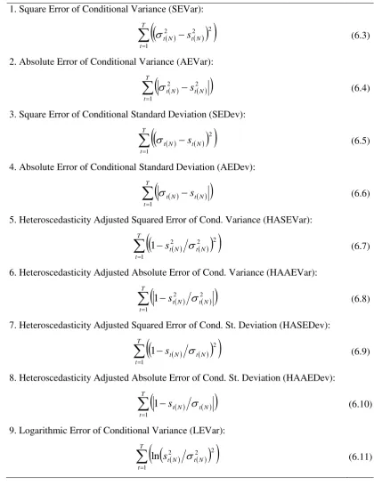
s , the following evaluation criteria are considered:

Squared Error (SE):



2_{ } 2_{ }



2

N t N t s

 (4.3

)

Absolute Error (AE): 2_{ } 2_{ }

N t N t s

 (4.4

)

Heteroscedasticity Adjusted Squared Error (HASE):



2_{ } 2_{ }



2

1stN t N

(4.5

)

Heteroscedasticity Adjusted Absolute Error (HAAE): 2_{ } 2_{ }

1stN t N (4.6

)

Logarithmic Error (LE):



2_{ } 2_{ }



2

lnstN tN (4.7

)

The first two functions have been widely used in the literature (see, e.g. Heynen and Kat

1994, West and Cho 1995, Yu 2002 and Brooks and Persand 2003). The HASE and HAAE

functions were considered by Walsh and Tsou (1998) and Andersen et al. (1999), while the

LE function was utilized by Pagan and Schwert (1990) and Saez (1997).

Usually, the average of the evaluation criteria is computed. However, when

simulating an AR(1)GARCH(1,1) process, which is the most commonly used model in

financial applications, the distributions of



2_{ } 2_{ }



N t N t s

 ,



₁ 2_{ } 2_{ }



N t N t

s 

 and

   



2 2



lnstN tN are asymmetric with extreme outliers. It would therefore be advisable to

compute both the mean and the median of the evaluation criteria. Figure 1 depicts the

histograms of the one-step forecast error distribution from the following simulated process:

(11)

5. E x a m i n i n g t h e P e r f o r m a n c e o f t h e S P E C M o d e l S e l e c t i o n

A l g o r i t h m

In this section, the ability of the SPEC model selection algorithm to lead to the

ARCH models that track closer future volatility is illustrated on a series of daily

log-returns. As follows from section 2, the return series can be modeled in the following form:

 



, ,...; , ,...; , ,...



1

, 0 ~ ,

2 1 2 1 2 1 2

1 0

  

 



 



 





t t t

t t

iid t t t t

t i

i t i t

g

N z z

y c c

y

  

 

 

 

 

(5.1

)

In the sequel, the above form is considered in connection with the ARCH models defined

by (2.5), (2.6) and (2.7), for  0,1,2,3,4, p0,1,2 and q1,2, thus yielding a total of

85 casesix. The first autoregressive order of the conditional mean accounts for the

non-synchronous trading. However, various orders are considered as, according to Hansen and

Lunde (2003), a small improvement of the modeling of the conditional mean, may lead to a

clear improvement in the forecast of volatility. Also, contrary to the majority of applied

studies, such as those by Klaassen (2002), Vilasuso (2002) and Hansen and Lunde (2003),

where the forecasts are calculated by estimating the models once, in the present study the

models are re-estimated every trading day, in order to evaluate the forecast accuracy under

real world circumstances. Further, as Degiannakis and Xekalaki’s (2005) results reveal, the SPEC algorithm can be applied to all the conditional variance functions with consistent

and asymptotically normal estimators of the parameters. Thus, although, austerely

mathematically, minimizing the sum of squared standardized one-step-ahead residuals is

not equivalent to maximizing the likelihood, Bollerslev and Wooldridge’s (1992) quasi -maximum likelihood method is employed in the sequel to estimate the models. Maximum

likelihood estimates of the parameters are obtained by numerical maximization of the

log-likelihood function using the Marquardt algorithm (Marquardt 1963), a modification of the

Berndt, Hall, Hall and Hausman, or BHHH, algorithm (Berndt et al. 1974). The

quasi-maximum likelihood estimator (QMLE) is used, as according to Bollerslev and

Wooldridge, it is generally consistent, has a normal limiting distribution and provides

asymptotic standard errors that are valid under non-normality.

The data set consists of 1661 S&P500 daily log-returns in the period from

November 24th, 1993 to June 26th, 2000. Although, large data sets are often used in the

literature for the estimation of ARCH models, we consider here using a not too large

sample, which would expectantly incorporate changes in trading behavior more efficiently

as the evidence is from various findings in the literature (e.g. Engle et al. 1993, Frey and

(12)

processes are estimated using a rolling sample of constant size equal to 500. Thus, the first

one-step-ahead volatility prediction, 2 | 1

ˆt t

 , is available at time t500. Applying the

SPEC model selection algorithm, the sum of squared standardized one-step-ahead

prediction errors,



_ 

T t 1ztt

2 1 |

ˆ , was estimated considering various values for T, and, in

particular, T 5

 

580x. Thus, the evaluation criteria were applied on the one-step-ahead forecasts using 1661500801081 data points, on the two-step-ahead forecasts using

1080 81 500

1661   data points, …, and on the Nth-step-ahead forecasts using

1

1081N data points.

Adopting Brooks and Persand’s (2003) approach we consider evaluating multi-step-ahead forecasts based on overlapping time periods. In particular, most of the studies in

the literature evaluate the multi-step forecasts using non-overlapping time periods in order

to infer about the statistical significance of the ranking. Our main purpose is to examine the

application potential of the SPEC algorithm of selection of models on the basis of their

forecasting ability in terms of volatility. So, the mean and the median value of each of the

5 evaluation criteria, in equations (4.3)-(4.7), were computed, yielding a total of 10

evaluation criteria for each forecasting horizon from one day to one hundred days ahead.

However, volatility is expressed either as the variance or as the standard deviation. Thus,

in order to examine possible differences between forecasting the variance and its square

root, the evaluation criteria were, also, applied on the standard deviation. Therefore, 2_{ }

N t



and st2_{ }N , in equations (4.3)-(4.7), were replaced by t N and st N , respectively and 10

more evaluation criteria were computed. In total, 20 evaluation criteria were computed for

a horizon ranging from one trading day to five trading months. In section 4.1, two realized

volatility measures were mentioned. As, qualitatively, they are of the same nature, in the

sequel, we base the analysis on the realized volatility as defined by st2_{ }N .

xi

It was examined whether the ARCH models selected by the SPEC algorithm

achieve the lowest value of the evaluation criteria. The main focus was on the median

values of the criteria and mainly on the heteroscedasticity adjusted criteria since they are

more robust to asymmetry. The comparative evaluation is performed by computing the loss

functions for variance forecasts always obtained by a single model on the one hand, and for

variance forecasts obtained by models picked by the SPEC algorithm on the other. Table 2,

(13)

algorithm achieves the minimum value of the evaluation criteria. The minARCH and

minSPEC values refer to the minima of the evaluation criteria achieved by a single model

and by models picked by the SPEC algorithm, respectively. As concerns the variance

forecasts obtained by any single model, the results are in line with those existing in the

literature, i.e. they are not consistent across all functions. Although, the exponential ARCH

specification exhibits the best performance in the majority of the cases (84.1% of the cases

presented in Table 2), the autoregressive order of the conditional mean is not constant

across the evaluation criteria. However, the lag order pq 1 of the EGARCH variance

specification exhibits the best performance in 63.4% of the cases.

Figure 2 shows, for each evaluation criterion and each forecasting horizon, whether

ARCH models selected by the SPEC algorithm achieve the lowest value of the evaluation

criteria. In the first part of Figure 2, the performance of the models, which are selected by

the SPEC algorithm, on the basis of the conditional variance is depicted, while, the second

part refers to their performance on forecasting standard deviation. The general conclusion

is that the SPEC algorithm leads to the selection of the ARCH processes which track closer

the realized volatility in the majority of the cases. Specifically, for the forecasting horizon

ranging from 11 to 52 days, the models selected by the SPEC algorithm achieve the lowest

criteria values, irrespectively of the evaluation criteria. The percentage of cases, in which

the models picked by the SPEC algorithm achieve the lowest value of the evaluation

criteria, is higher around the forecasting horizon ranging from 16 to 36 days ahead, or 4 to

7 trading weeks ahead. The result is in accordance to Degiannakis and Xekalaki (2001)

who provided evidence that option’s traders using variance forecasts for horizons ranging from ten to forty trading days obtained by models suggested by the SPEC algorithm

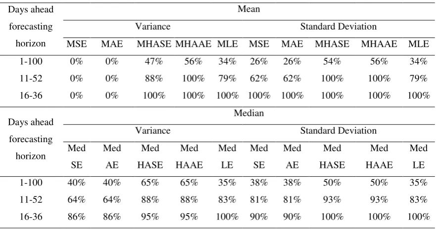
achieved the highest rate of return among a set of model selection criteria. Table 3 presents

the percentage of cases the models selected by the SPEC algorithm perform “better” than

any other single model as judged by the evaluation criteria, for 3 different horizon ranges.

Note that, in terms of the MSE and MAE criteria, none of the models chosen by the SPEC

algorithm appears to perform better in any of the forecasting horizons considered. But, in

terms of the median values of the criteria and the heteroscedasticity adjusted criteria, which

are robust to asymmetry, the models selected by the SPEC algorithm appear to have a

better performance than any other single model in all the forecasting horizons.

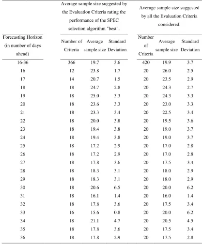
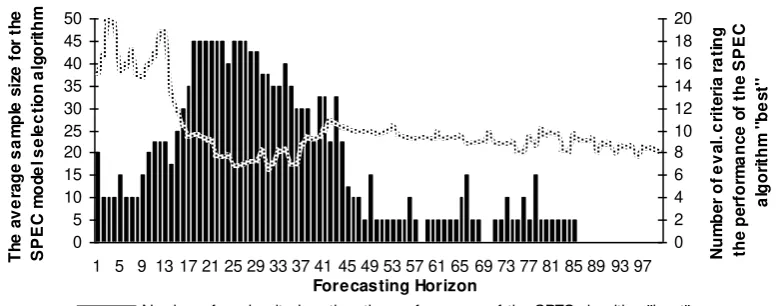
It is interesting to note that, via the evaluation criteria, the suggested sample size,

T, for the SPEC model selection algorithm can be determined. The SPEC model selection

algorithm has been applied for T 5

 

580. In the sequel, the value of T for which the SPEC selection method achieves the best performance according to the evaluation criteria

(14)

criteria, across the forecasting horizons. The bar charts are a graphical representation of the

number of evaluation criteria by which the performance of the models selected by the

SPEC algorithm were judged “better” than the performance of any other single model (measured on the right hand side vertical axis). For a 16 to 36 days ahead forecasting

horizon, the appropriate T, as concerns the specific data, ranges around 20 days with a

standard deviation of 3.6 days. Table 4 provides more details for the sample size of the

SPEC selection method suggested by the evaluation criteria and its standard deviation for

both the entire 16 to 36 day ahead forecasting horizon and for each day individually. The

SPEC model selection algorithm shows a better performance for a sample size of about 20

days.

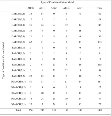
Several results in the literature (e.g. Lopez and Walter 2001, Christoffersen and

Jacobs 2003 and Ferreira and Lopez 2003) reveal that the simplest model specifications are

chosen a disproportionately large percentage of the time, while others (e.g. Vilasuso 2002,

Brooks and Persand 2003, Hansen and Lunde 2003, Giot and Laurent 2003, 2004,

Angelidis et al. 2004, Degiannakis 2004) indicate that the more flexible an ARCH model

is, the more adequate it is in volatility forecasting, compared to parsimonious models. In

order to give the reader a sense of which of the 85 models was selected most often, Table 5

presents the models selected by the SPEC(20) algorithm. For example, the model with

AR(0) conditional mean and GARCH(0,1) conditional variance was picked on 34 trading

days. As concerns the conditional variance function, the GARCH, EGARCH and TARCH

models were picked as the most suitable in the 38%, 39%, and 23% of the cases,

respectively. On the basis of the results of Table 5, the SPEC algorithm does not appear to

be noticeably biased towards selecting a specific type of model. This is in line with

Degiannakis and Xekalaki’s (2001) findings. Tables for the remaining sample sizes T of the SPEC algorithm were also constructed giving qualitatively similar resultsxii.

6. C o m p a r i s o n o f t h e S P E C C r i t e r i o n t o O t h e r M e t h o d s o f

M o d e l S e l e c t i o n

Most of the methods used in the time series literature for selecting the appropriate

model are based on evaluating the ability of the models to describe the data. Standard

model selection criteria such as the Akaike information criterion [AIC] (Akaike 1973) and

the Schwarz Bayesian criterion [SBC] (Schwarz 1978) have widely been used in the

ARCH literature, despite the fact that their statistical properties in the ARCH context are

(15)

maximized value of the log-likelihood function of a model, where ˆ is the maximum

likelihood estimator of the parameter vector  based on a sample of size n and  denotes the dimension of  , thus:

 

 

ln ˆ

AIC (6.1)

 

ˆ 2 1 ln

 

n .

l

SBC  _n    (6.2)

In addition, model selection is mainly based on the evaluation of some loss

functions for each of the competing models. In this section, the statistical criteria, which

were considered in section 4 as measures in evaluating the predictive performance of a

variance model, are considered as criteria for the selection of ARCH models. In particular,

the model selection methods presented in Table 6 are considered and their ability to predict

future volatility is investigated.

Applying the SPEC algorithm, the sum of squared standardized one-step-ahead

prediction errors,



_  

T

t 1 tt tt 2 1 | 2

1

| ˆ

ˆ 

 , was estimated considering various values for T.

Therefore, each of the model selection criteria, in Table 6, was computed considering

various values for T, and, in particular, T 10

 

1080. The AIC and SBC criteria were computed based on the rolling sample of constant size equal to 500, or n500, that is

used at each time to estimate the parameters of the models. Selecting a strategy for each

method of model selection naturally amounts to selecting the model, which, at time k, has

the lowest value of the formula is indicated in Table 6.

As concerns the AIC and SBC selection methods, they do not achieve the lowest

value of the evaluation criteria in almost all the cases, which is indicative of the inability of

the in-sample model selection methods to suggest the models with superior volatility

forecasting performance. The general conclusion is that the loss functions presented in

Table 6 do not lead to the selection of the ARCH processes which track closer the realized

volatility. The HAAEVar, HASEVar and HASEDev methods show a better performance,

as they select the ARCH models with the lowest value of the evaluation criteria, around the

forecasting horizon ranging from 16 to 36 days ahead. So, they might be used in selecting

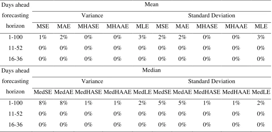
that model that generates “better” volatility predictions. The other selection methods failed

to pick the models that perform “better” in almost all the cases. Ιndicatively, Table 7 presents the percentage of cases the models selected by the HAAEVar and LEVar model

selection methods perform “better” as judged by the evaluation criteria. The performance

of the HASEVar and HASEDev selection methods is similar to that of the HAAEVa

rmethod, whereas the performance of the remaining methods is similar to that of the

(16)

order to investigate whether the suggested model selection method indicates the ARCH

models that track closer the realized volatility, the predictive ability of these loss functions

must be compared to the volatility forecasting ability of the SPEC criterion, and mainly for

a forecasting horizon ranging from 16 days to 36 days ahead.

Of main interest is whether the ARCH models selected by the SPEC algorithm

yield values for the evaluation criteria that are lower than those corresponding to the

ARCH models selected by the model selection methods summarized in Table 6. As

concerns forecasting horizons of 4 to 7 trading weeks ahead the performance of the SPEC

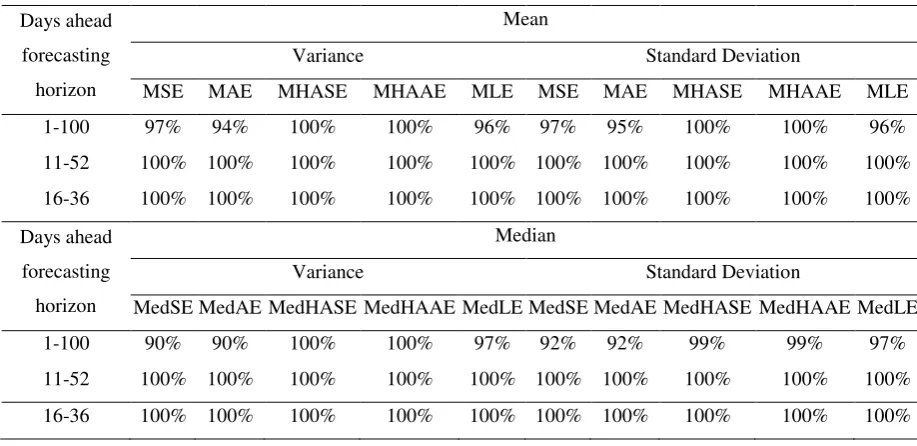
algorithm is by far the best. Table 8 presents, indicatively, the percentage of times the

ARCH models selected by the SPEC algorithm achieve lower values for the corresponding

evaluation criteria and the specific forecasting horizons than the models selected by the

HAAEVar and LEVar model selection methods. The SPEC algorithm performs “better”

than the other methods of model selection in about 90% of the cases. This percentage is

lower when the SPEC algorithm is compared to the HAAEVar, HASEVar and HASEDev

methods. Nevertheless, even in such cases, the opponent methods select the ARCH models

that track closer future volatility much less frequently than the SPEC algorithm. The

percentage of times, an opponent to the SPEC algorithm selects the most appropriate

models in forecasting future volatility, is highest in the case of the HAAEVar method.

However, only in the 23% of the cases, the ARCH models selected by the HAAEVar

method perform "better" than the models selected by the SPEC criterion, for any of the 3

horizon ranges. The performance of the remaining model selection methods is similar to

that of the LEVar method. Full tables with the comparison of all the model selection

methods to the SPEC algorithm are available upon request.

7. D i s c u s s i o n

The SPEC method, for selecting an ARCH model among several competing

models, amounts to choosing the model with the lowest sum of squared standardized

one-step-ahead forecasting errors. It incorporates the idea of “jumping” from one model to another, as stock market behavior alters. Thus, using the SPEC model selection algorithm

every time a volatility forecast is required, allows shifting from the model used to predict

the conditional variance the previous time to another.

In this paper, a number of evaluation criteria, for forecasting horizons ranging from

one day to one hundred days ahead, were applied and it was found that the ARCH models,

(17)

Brooks and Persand’s (2003) evaluation approach was adopted and multi -step-ahead forecasts were evaluated based on overlapping time periods. Alternatively, one

might like to consider non-overlapping time periods and apply other evaluation schemes,

such as those proposed by Diebold and Mariano (1995), Hansen and Lund (2003) or

Hansen et al. (2003).

A topic worth exploring is the application of SPEC algorithm on models that

account for recent developments in the area of volatility. Considering fractional integration

of the conditional variance, for example, is an interesting question with regard to

investigating SPEC’s applicability further. (For more details, see, e.g., Giot and Laurent

2003 and Degiannakis 2004). Finally, assessing the utility of the SPEC algorithm as a tool

in model selection for ARCH models with non-normally distributed conditional

innovations would be equally worthy as it would bring into play more general forms of

models in the statistical and econometric literature.

R e f e r e n c e s

Adrangi, B. and Chatrath, A. (2003). Non-Linear Dynamics in Futures Prices: Evidence

From the Coffee, Sugar and Cocoa Exchange. Applied Financial Economics, 13,

245-256.

Akaike, H. (1973). Information Theory and an Extension of the Maximum Likelihood

Principle. Proceedings of the second international symposium on information theory.

B.N. Petrov and F. Csaki (eds.), Budapest, 267-281.

Alizabeh, S., Brandt M.W. and Diebold, F.X. (2002). Range-Based Estimation of Stochastic

Volatility Models. Journal of Finance, LV11, 1047-1091.

Andersen, T. and Bollerslev, T. (1997). Intraday Periodicity and Volatility Persistence in

Financial Markets. Journal of Empirical Finance, 4, 115-158.

Andersen, T. and Bollerslev, T. (1998a). Answering the Skeptics: Yes, Standard Volatility

Models Do Provide Accurate Forecasts. International Economic Review, 39, 885-905.

Andersen, T. and Bollerslev, T. (1998b). DM-Dollar Volatility: Intraday Activity Patterns,

Macroeconomic Announcements and Longer-Run Dependencies. Journal of Finance,

53, 219-265.

Andersen, T., Bollerslev, T. and Lange, S. (1999). Forecasting Financial Market Volatility:

Sample Frequency vis-à-vis Forecast Horizon. Journal of Empirical Finance, 6, 457-477.

Andersen, T., Bollerslev T. and Cai, J. (2000a). Intraday and Interday Volatility in the

Japanese Stock Market. Journal of International Financial Markets, Institutions and

(18)

Andersen, T., Bollerslev, T., Diebold, F.X. and Labys, P. (2000b). Exchange Rate Returns

Standardized by Realized Volatility are (Nearly) Gaussian. Multinational Finance

Journal, 4, 159-179.

Andersen, T., Bollerslev, T., Diebold, F.X. and Labys, P. (2001a). The Distribution of

Exchange Rate Volatility. Journal of the American Statistical Association, 96, 42-55.

Andersen, T., Bollerslev, T., Diebold, F.X. and Ebens, H. (2001b). The Distribution of

Stock Return Volatility. Journal of Financial Economics, 61, 43-76.

Andersen, T., Bollerslev, T., Diebold, F.X. and Labys, P. (2003). Modeling and

Forecasting Realized Volatility. Econometrica, 71, 529-626.

Andersen, T., Bollerslev, T. and Diebold, F.X. (2005). Parametric and Nonparametric

Volatility Measurement. Handbook of Financial Econometrics, (eds.) Yacine Aït

-Sahalia and Lars Peter Hansen, Amsterdam, North Holland.

Angelidis, T., Benos, A. and Degiannakis, S. (2004). The Use of GARCH Models in VaR

Estimation. Statistical Methodology, 1, 1(2), 105-128.

Barkoulas, J. and Travlos, N. (1998). Chaos in an Emerging Capital Market? The Case of

the Athens Stock Exchange. Applied Financial Economics, 8, 231-243.

Barkoulas, J., Baum, C.F. and Travlos, N. (2000). Long Menory in the Greek Stock Market.

Applied Financial Economics, 10, 177-184.

Barndorff-Nielsen, O.E. and Shephard, N. (1998). Aggregation and Model Construction

for Volatility Models. University of Aarhus and Nuffield College, Oxford, Department

of Mathematical Sciences, Manuscript.

Basle Committee on Banking Supervision. (1998). International Convergence of Capital

Measurement and Capital Standards.

Bera, A.K. and Higgins, M.L. (1993). ARCH Models: Properties, Estimation and Testing.

Journal of Economic Surveys, 7, 305-366.

Berndt, E.R., Hall, B.H. Hall, R.E. and Hausman, J.A. (1974). Estimation and Inference in

Nonlinear Structural Models. Annals of Economic and Social Measurement, 3, 653-665.

Bollerslev, T. (1986). Generalized Autoregressive Conditional Heteroskedasticity. Journal

of Econometrics, 31, 307–327.

Bollerslev, T. and Wooldridge, J.M. (1992). Quasi-maximum Likelihood Estimation and

Inference in Dynamic Models with Time-Varying Covariances. Econometric Reviews,

11, 143-172.

(19)

Bollerslev, T., Engle, R.F. and Nelson, D. (1994). ARCH Models, in Handbook of

Econometrics, Volume 4, eds. R. Engle and D. McFadden, Elsevier Science,

Amsterdam, 2959-3038.

Brock, W. (1986). Distinguishing Random and Deterministic Systems: Abridged Version,

Journal of Economic Theory, 40, 168-195.

Brock, W.A., Dechert, W.D. and Scheinkman, J.A. (1987). A Test for Independence Based

on the Correlation Dimension. Department of Economics, University of Wisconsin,

Madison, WI. SSRI, Working Paper no. 8702.

Brooks, C. and Persand, G. (2003). The effect of asymmetries on stock index return

Value-at-Risk estimates. The Journal of Risk Finance, Winter, 29-42.

Campbell, J., Lo, A. and MacKinlay, A.C. (1997). The Econometrics of Financial Markets.

New Jersey. Princeton University Press.

Christoffersen, P. and Jacobs, K. (2003). Which Volatility Model for Option Evaluation?,

Faculty of Management, McGill University, Manuscript.

Cohen, K., Hawawini, G., Maier, S., Schwartz, R. and Whitcomb, D. (1983). Friction in

the Trading Process and the Estimation of Systematic Risk. Journal of Financial

Economics, 12, 263-278.

Degiannakis, S. (2004). Volatility Forecasting: Evidence from a Fractional Integrated

Asymmetric Power ARCH Skewed-t Model. Applied Financial Economics, 14,

1333-1342.

Degiannakis, S. and Xekalaki, E. (2001). Using a Prediction Error Criterion for Model

Selection in Forecasting Option Prices. Technical Report no 131, Department of

Statistics, Athens University of Economics and Business.

(http://stat-athens.aueb.gr/~exek/papers/Xekalaki-TechnRep131(2001)ft.pdf )

Degiannakis, S. and Xekalaki, E. (2004). Autoregressive Conditional Heteroscedasticity

Models: A Review. Quality Technology and Quantitative Management, 1, (2), 271-324.

Degiannakis, S. and Xekalaki, E. (2005). Predictability and Model Selection in the Context

of ARCH Models. Journal of Applied Stochastic Models in Business and Industry, 21,

55-82.

Diebold, F.X. and Mariano, R. (1995). Comparing Predictive Accuracy, Journal of

Business and Economic Statistics, 13, 3, 253-263.

Dimson, E. (1979). Risk Measurement When Shares Are Subject to Infrequent Trading.

Journal of Financial Economics, 7, 197-226.

Ebens, H. (1999). Realized Stock Volatility. Department of Economics, Johns Hopkins

(20)

Engle, R.F., Hong, C.H., Kane, A. and Noh, J. (1993). Arbitrage Valuation of Variance

Forecasts with Simulated Options, Advances in Futures and Options Research, 6,

393-415.

Ferreira, M.A. and Lopez, J.A. (2003). Evaluating Interest Rate Covariance Models within

a Value-at-Risk Framework. Economic Research Department, Federal Reserve Bank of

San Francisco, manuscript.

Franses, P.H. and Homelen, P.V. (1998). On Forecasting Exchange Rates Using Neural

Networks. Applied Financial Economics, 8, 589-596.

Frey, R. and Michaud, P. (1997). The Effect of GARCH-type Volatilities on Prices and

Payoff-Distributions of Derivative Assets - a Simulation Study, ETH Zurich, Working

Paper.

Giot, P. and Laurent, S. (2003). Value-at-Risk for Long and Short Trading Positions.

Journal of Applied Econometrics, 18, 641-664.

Giot, P. and Laurent, S. (2004). Modelling Daily Value-at-Risk Using Realized Volatility

and ARCH Type Models. Journal of Empirical Finance, 11, 379-398.

Glosten, L., Jagannathan, R. and Runkle, D. (1993). On the Relation Between the Expected

Value and the Volatility of the Nominal Excess Return on Stocks. Journal of Finance,

48, 1779–1801.

González-Rivera, G., Lee, T-H and Mishra, S. (2004). Forecasting Volatility: A Reality Check Based on Option Pricing, Utility Function, Value-at-Risk and Predictive

Likelihood. International Journal of Forecasting, 20, 629-645.

Gourieroux, C. (1997). ARCH models and Financial Applications. Springer-Verlag, New

York.

Hamilton, J. (1994). Time Series Analysis, New Jersey: Princeton University Press

Hansen, P.R. and Lunde, A. (2003). A Forecast Comparison of Volatility Models: Does

Anything Beat a GARCH(1,1)? Brown University, Department of Economics, Working

Paper.

Hansen, P.R., Lunde, A. and Nason, J.M. (2003). Choosing the Best Volatility Models:

The Model Confidence Set Approach. Brown University, Department of Economics,

Working Paper.

Hecq, A. (1996). IGARCH Effect on Autoregressive Lag Length Selection and Causality

Tests. Applied Economics Letters, 3, 317-323.

(21)

Hol, E. and Koopman, S. (2000). Forecasting the Variability of Stock Index Returns with

Stochastic Volatility Models and Implied Volatility. Tinbergen Institute, Discussion

Paper No. 104,4.

Holden, A. (1986). Chaos, New Jersey: Princeton University Press.

Hsieh, D. (1991). Chaos and Nonlinear Dynamics: Application to Financial Markets,

Journal of Finance, 46, 1839-1877.

Hutchinson, J., Lo, A. and Poggio, T. (1994). A Nonparametric Approach to the Pricing

and Hedging of Derivative Securities Via Learning Networks, Journal of Finance, 49,

851-889.

Jasic, T. and Wood, D. (2004). The Profitablity of Daily Stock Market Indices Trades Based

on Neural Network Predictions: Case Study for the S&P500, the DAX, the TOPIX and

the FTSE in the Period 1965-1999. Applied Financial Economics, 14, 285-297.

Kibble, W. F. (1941). A Two Variate Gamma Type Distribution. Sankhya, 5, 137-150.

Klaassen, F. (2002). Improving GARCH Volatility Forecasts With Regime-Switching

GARCH, in Advances in Markov-Switching Models, eds. J.D. Hamilton and B. Raj,

Psysica Verlag, New York, 223-254.

Lo, A. and MacKinlay, A.C. (1988). Stock Market Prices Do Not Follow Random Walks:

Evidence from a Simple Specification Test. Review of Financial Studies, 1, 41-66.

Lo, A. and MacKinlay, A.C. (1990). An Econometric Analysis of Non-synchronous

Trading. Journal of Econometrics, 45, 181-212.

Lopez, J.A. and Walter, C.A. (2001). Evaluating Covariance Matrix Forecasts in a

Value-at-Risk Framework. Journal of Risk, 3, 3, 69-98.

Marquardt, D.W. (1963). An Algorithm for Least Squares Estimation of Nonlinear

Parameters. Journal of the Society for Industrial and Applied Mathematics, 11, 431-441.

Nelson, D. (1991). Conditional Heteroskedasticity in Asset Returns: A New Approach.

Econometrica, 59, 347-370.

Pagan, A.R. and Schwert, G.W. (1990). Alternative Models for Conditional Stock

Volatility. Journal of Econometrics, 45, 267-290.

Peel, D.A. and Speight, A.E.H. (1996). Is the US Business Cycle Asymmetric? Some

Further Evidence. Applied Economics, 28, 405-415.

Perez-Rodriguez, J.V., Torra, S. and Andrada-Felix, J. (2005). Are Spanish Ibex35 Stock

Future Index Returns Forecasted with Non-Linear Models? Applied Financial

Economics, 15, 963-975.

Plasmans, J., Verkooijen, W. and Daniels, H. (1998). Estimating Structural Exchange Rate

(22)

Poggio, T. and Girosi, F. (1990). Networks for Approximation and Learning, Proceeding

of the IEEE, special issue: Neural Networks I: Theory and Modeling, 78, 1481-1497.

Priestley, M. (1988). Nonlinear and Non-Stationary Time Series Analysis, Academic

Press, San Diego.

Sadorsky, P. (2005). Stochastic Volatility Forecasting and Risk Management. Applied

Financial Economics, 15, 121-135.

Saez, M. (1997). Option Pricing Under Stochastic Volatiltiy and Stochastic Interest Rate in

the Spanish Case. Applied Financial Economics, 7, 379-394.

Saltoglu, B. (2003). Comparing Forecasting Ability of Parametric and Non-Parametric

Methods: An Application with Canadian Monthly Interest Rates. Applied Financial

Economics, 13, 169-179.

Scholes, M. and Williams, J. (1977). Estimating Betas from Non-Synchronous Data.

Journal of Financial Economics, 5, 309-328.

Schwarz, G. (1978). Estimating the Dimension of a Model. Annals of Statistics, 6,

461-464.

Selcuk, F. (2005). Asymmetric Stochastic Volatility in Emerging Stock Market. Applied

Financial Economics, 15, 867-874.

Shephard, N. (1996). Statistical Aspects of ARCH and Stochastic Volatility Models. In

Time Series Models in Econometrics, Finance and Other Fields, 1-67, (eds.) D.R. Cox,

D.V. Hinkley and O.E. Barndorff-Nielsen, Chapman & Hall, London.

Taylor, S.J. (1994). Modelling Stochastic Volatility: A Review and Comparative Study.

Mathematical Finance, 4, 183-204.

Teräsvirta, T., Tjǿstheim, D. and Granger, C. (1994). Aspects of Modeling Nonlinear Time

Series, in Handbook of Econometrics, Volume 4, eds. R. Engle and D. McFadden,

Elsevier Science, Amsterdam.

Thompson, J. and Stewart, H. (1986). Nonlinear Dynamics and Chaos, John Wiley and

Sons, NY.

Tong, H. (1990). Nonlinear Time Series: A Dynamic System Approach, Oxford University

Press, Oxford.

Vilasuso, J. (2002). Forecasting Exchange Rate Volatility. Economics Letters, 76, 59-64.

Walsh, D.M. and Tsou, G. Y.-G. (1998). Forecasting Index Volatility: Sampling Interval

and Non-Trading Effects. Applied Financial Economics, 8, 477-485.

(23)

White, H. (1992). Artificial Neural Networks: Approximation and Learning Theory,

Blackwell Publishers, Cambridge, MA.

Xekalaki, E. and Degiannakis, S. (2005). Evaluating Volatility Forecasts in Option Pricing

in the Context of a Simulated Options Market. Computational Statistics and Data

Analysis. Special Issue on Computational Econometrics, forthcoming.

Xekalaki E., Panaretos, J. and Psarakis, S. (2003). A Predictive Model Evaluation and

Selection Approach - The Correlated Gamma Ratio Distribution. Stochastic Musings:

Perspectives from the Pioneers of the Late 20th Century, (J. Panaretos, ed.), Lawrence Erlbaum, Associates Publishers, 188-202.

Yu, J. (2002). Forecasting Volatility in the New Zealand Stock Market. Applied Financial

(24)

Table 1. The estimation steps required at time k for each model m by the

SPEC model selection algorithm. At time k (k T,T1,...), select the model

m with the minimum value for the sum of the squares of the T most recent

standardized one-step-ahead prediction errors,



 



   

         k T k t m t t m t t k T k t m t z 1 2 1 | 2 1 | 1

2 ˆ ˆ

ˆ   .

[image:24.595.151.514.160.397.2]

(25)

[image:25.595.115.557.169.402.2]

Table 3. The percentage of times the ARCH models selected by the SPEC algorithm perform "better" than any other single model as judged by the evaluation criteria. The first and the second panel correspond to the mean and the median of the evaluation criteria, respectively. The left and the right part of the panels correspond to the volatility expressed as the variance and the standard deviation of the returns, respectively.

Days ahead forecasting horizon

Mean

Variance Standard Deviation

MSE MAE MHASE MHAAE MLE MSE MAE MHASE MHAAE MLE 1-100 0% 0% 47% 56% 34% 26% 26% 54% 56% 34% 11-52 0% 0% 88% 100% 79% 62% 62% 100% 100% 79% 16-36 0% 0% 100% 100% 100% 100% 100% 100% 100% 100%

Days ahead forecasting horizon

Median

Variance Standard Deviation

Med SE

Med AE

Med HASE

Med HAAE

Med LE

Med SE

Med AE

Med HASE

Med HAAE

Med LE 1-100 40% 40% 65% 65% 35% 38% 38% 50% 50% 35% 11-52 64% 64% 88% 88% 83% 81% 81% 93% 93% 83% 16-36 86% 86% 95% 95% 100% 90% 90% 100% 100% 100%

MSE: Mean Square Error MAE: Mean Absolute Error

MHASE: Mean Heteroscedasticity Adjusted Squared Error MHAAE: Mean Heteroscedasticity Adjusted Absolute Error MLE: Mean Logarithmic Error

MedSE: Median Square Error MedAE: Median Absolute Error

MedHASE: Median Heteroscedasticity Adjusted Squared Error MedHAAE: Median Heteroscedasticity Adjusted Absolute Error

(26)

Table 4. Average sample size for the SPEC model selection algorithm suggested by the evaluation criteria for both the entire 16 to 36 days ahead forecasting horizon and for each day individually.

Average sample size suggested by the Evaluation Criteria rating the

performance of the SPEC selection algorithm "best".

Average sample size suggested by all the Evaluation Criteria

considered.

Forecasting Horizon (in number of days

ahead)

Number of Criteria

Average sample size

Standard Deviation

Number of Criteria

Average sample size

Standard Deviation