Melissa: Bayesian clustering and imputation of single cell methylomes

M E T H O D

Open Access

Melissa: Bayesian clustering and

imputation of single-cell methylomes

Chantriolnt-Andreas Kapourani

and Guido Sanguinetti

Abstract

Measurements of single-cell methylation are revolutionizing our understanding of epigenetic control of gene expression, yet the intrinsic data sparsity limits the scope for quantitative analysis of such data. Here, we introduce Melissa (MEthyLation Inference for Single cell Analysis), a Bayesian hierarchical method to cluster cells based on local methylation patterns, discovering patterns of epigenetic variability between cells. The clustering also acts as an effective regularization for data imputation on unassayed CpG sites, enabling transfer of information between individual cells. We show both on simulated and real data sets that Melissa provides accurate and biologically meaningful clusterings and state-of-the-art imputation performance.

Background

DNA methylation is probably the best studied epige-nomic mark, due to its well-established heritability and widespread association with diseases and a broad range of biological processes, including X-chromosome inacti-vation, cell differentiation, and cancer progression [1–3]. Yet its role in gene regulation, and the molecular mech-anisms underpinning its association with diseases, is still imperfectly understood.

Bisulfite treatment of DNA followed by sequencing (BS-seq) has provided a powerful tool for measuring the methylation level of cytosines on a genome-wide scale with single nucleotide resolution [4]. BS-seq protocols have been vastly improved over the last decade, with BS-seq rapidly becoming a widespread tool in biomedi-cal investigation. Nevertheless, until very recently, BS-seq could only be used to measure methylation in bulk pop-ulations of cells [5], preventing effective investigations of the role of DNA methylation in shaping transcriptional variability and early development [6,7].

This shortcoming has been addressed within the last 5 years through the development of protocols to measure DNA methylation at single-cell resolution using either scBS-seq [8] or scRRBS [9] making it possible to uncover

*Correspondence:[email protected];[email protected]

1_{School of Informatics, University of Edinburgh, Edinburgh EH8 9AB, UK} 2_{MRC Institute of Genetics and Molecular Medicine, University of Edinburgh,} Edinburgh EH4 2XU, UK

Full list of author information is available at the end of the article

the heterogeneity and dynamics of DNA methylation [10]. Even more recently, methods have been developed that can sequence both the methylome and the transcriptome or other features in parallel, potentially enabling a quan-tification of the role of DNA methylation in explaining transcriptional heterogeneity [11–13]. However, due to the small amounts of genomic DNA per cell, these pro-tocols usually result in very sparse genome-wide CpG coverage (i.e., for most CpGs, we have missing values), ranging from 5% in high-throughput studies [14, 15] to 20% in low-throughput ones [8,11]. The sparsity of the data represents a major hurdle to effectively use single-cell methylation assays to inform our understanding of epigenetic control of transcriptomic variability, or to dis-tinguish individual cells based on their epigenomic state.

In this paper, we address these problems by using a two-pronged strategy. First, we note that several recent studies have highlighted the importance of local methyla-tion profiles, as opposed to individual CpG methylamethyla-tion, in determining the epigenetic state of a region [16–18]. This implies that local spatial correlations may be effec-tively leveraged to ameliorate the issue of data sparsity. Secondly, single-cell BS-seq protocols, as all single-cell high-throughput protocols, simultaneously assay a large number of cells, ranging from several tens [8] to a few thousands in the most recent studies [14]. Such abun-dance of data could be exploited to our advantage to transfer information across similar cells.

We implement both of these strategies within Melissa (MEthyLation Inference for Single cell Analysis), a Bayesian hierarchical model that jointly learns the methy-lation profiles of genomic regions of interest and clusters cells based on their genome-wide methylation patterns. In this way, Melissa can effectively use both the informa-tion of neighboring CpGs and of other cells with similar methylation patterns in order to predict CpG methyla-tion states. As an addimethyla-tional benefit, Melissa also provides a Bayesian clustering approach capable of identifying subsets of cells based solely on epigenetic state, to our knowledge the first clustering method tailored specifi-cally to this rapidly expanding technology. We benchmark Melissa on both simulated and real single-cell BS-seq data, demonstrating that Melissa provides both state-of-the art imputation performance and accurate clustering of cells. Furthermore, thanks to a fast variational Bayes estimation strategy, Melissa has good scalability and can provide an effective modeling tool for the increasingly large single-cell methylation studies which will become prevalent in coming years.

Results and discussion

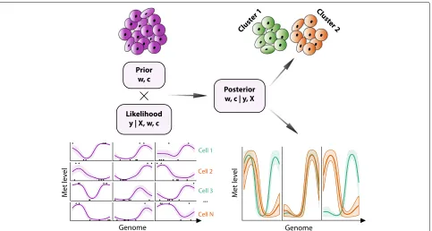
Melissa addresses the data sparsity issue by leveraging local correlations between neighboring CpGs and simi-larity between individual cells (see Fig. 1). The starting point is the definition of a set of genomic regions (e.g.

genes or enhancers) over which the model will be applied. Within each region, Melissa postulates a latent profile of methylation, a function mapping each CpG within the region to a number in [ 0, 1] which defines the proba-bility of that CpG being methylated. To ensure spatial smoothness of the profile, Melissa uses a generalized lin-ear model (GLM) of basis function regression along the lines of [16] (with modified likelihood to account for single cell data). Local correlations are however often insufficient for regions with extremely sparse coverage, and these are quite common in scBS-seq data. Therefore, we share information across different cells by coupling the local GLM regressions through a shared prior dis-tribution. In order to respect the (generally unknown) population structure that may be present within the cells assayed, we choose a (finite) Dirichlet mixture model prior. The output of Melissa is therefore twofold: at each genomic region in each cell, we get a predicted pro-file of methylation, which can be used to impute miss-ing data (i.e., unassayed CpGs). For each cell, we also get a discrete cluster membership probability, provid-ing a methylome-based clusterprovid-ing of cells. This twofold output of Melissa reflects its methodological founda-tions as a hybrid between a global unsupervised model (Bayesian clustering of methylomes) and a local super-vised learning model (GLM regression for every region). In this sense, Melissa is closer to a mixture of experts

model [19, Chapter 14, Section 5] than a standard mixture model.

Benchmarking Melissa on simulated data

We benchmark the ability of our model to cluster and impute CpG methylation states at the single-cell level both on simulated and mouse embryonic stem cell (ESC) data sets. To assess test prediction performance, we consider different metrics, includingF-measure, the area under the receiver operating characteristic curve (AUC), and preci-sion recall curves [20]. We explore the performance of a number of methods as we vary three possible experimen-tal parameters: the number of cells assayed, the cluster dissimilarity (how different the methylomes of cells in dif-ferent clusters are expected to be), and the CpG coverage (defined as the fraction of CpG sites covered by at least one read, averaged over all cells).

To benchmark the performance of Melissa in predicting CpG methylation states, we compare it against six dif-ferent imputation strategies. As a baseline approach, we compute the average methylation rate separately for each cell and region (Rate), that is, the average is taken over all CpG sites forming a genomic region. We also use the BPRMeth model [16,21], where we account for the binary nature of the observations, which we train independently across cells and regions (BPRMeth). Note that BPRMeth shares information across CpG sites inside each genomic region; however, it does not transfer information across cells. To share information across cells, but not across neighboring CpGs inside the region, we constrain Melissa to infer constant functions, i.e., learn average methyla-tion rate (Melissa rate). We also use a Gaussian mixture model (GMM) that takes as input averageMvalues [22] instead of average methylation rates across the region (see the “Methods” section); to avoid possible problems due to high-dimensionality, the GMM method was also tested on reduced-dimensionality data, where the first ten principal components were retained. Additionally, as a fully independent baseline, we use a Random Forest clas-sifier trained on individual cells and regions, where the input features are the observed CpG locations, and the response variable is the CpG methylation state: methy-lated or unmethymethy-lated (RF). This is essentially the method of [23], however, without using additional annotation data or DNA sequence patterns. We delay comparisons with the deep learning method DeepCpG [24] to the next section, as DeepCpG is not applicable in the settings of this simulation (see below).

In order to generate realistic simulated single-cell DNA methylation data, we extracted methylation profiles from real (bulk) BS-seq data using the BPRMeth package [21], and then generated binary methylation levels at a random subset of CpGs to simulate the low coverage of scBS-seq. In total, we simulated N = 200 cells fromK = 4

sub-populations, where each cell consisted ofM = 100 genomic regions. Additionally, to account for different levels of similarity between cell sub-populations, we sim-ulated 11 different data sets by varying the proportion of similar genomic regions between clusters. Finally, to assess the performance of Melissa as a function of assayed single cells, we simulated 10 different data sets by vary-ingN, the total number of single cells (see the “Methods” section).

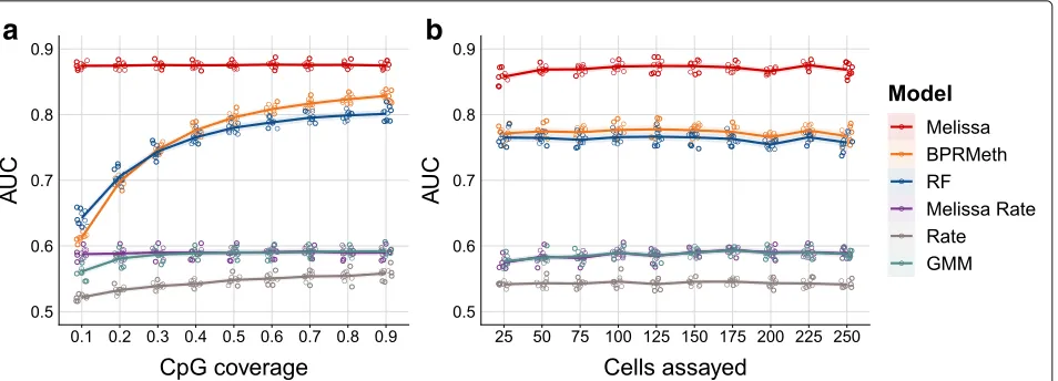
Applying the competing methods to synthetic data, we observe that Melissa yields a substantial improvement in prediction accuracy compared to all other models (Fig.2, Additional file1: Figure S1 and S2). Notably, Melissa is robust across different settings of the data, such as CpG coverage proportion (Fig.2a) or the total number of cells assayed in each experiment (Fig.2b). Due to its ability to transfer information across cells and neighboring CpGs, our model robustly maintains its prediction accuracy at a very sparse coverage level of 10% or even when assaying around 25 single cells. TheBPRMethandRFmodels per-form poorly at low CpG coverage settings, becoming com-parable to Melissa when using the majority of the CpGs for training set. Importantly, Melissa still performs better at 90% CpG coverage, demonstrating that the clustering acts as an effective regularization for imputing unassayed CpG sites. As expected, Melissa Rate and GMM have very similar performance (due to the very similar model structure); for both methods, performance is significantly weaker thanMelissa across the full range of simulation settings, since they are not expressive enough to cap-ture spatial correlations between CpGs. Using GMM on reduced dimensionality data did not lead to an improve-ment in performance, either for imputation or clustering (data not shown). Finally, the naive Rate method has the worst imputation performance of all methods, by a considerable margin. The imputation performance of all methods is relatively insensitive to the degree of cluster dissimilarity (Additional file1: Figure S2).

a

b

Fig. 2Melissa robustly imputes CpG methylation states.aImputation performance in terms of AUC as we vary the proportion of covered CpGs used for training. Higher values correspond to better imputation performance. For each CpG coverage setting, a total of 10 random splits of the data to training and test sets was performed. Each colored circle corresponds to a different simulation. The plot shows also the LOESS curve for each method as we increase CpG coverage. The methods considered wereMelissawhich shares information across cells and neighboring CpGs, the BPRMethmodel that only shares information across neighboring CpGs, and a Random Forest classifier (RF) which predicts CpG methylation states using as input the observed CpG locations. Additionally, we considered three baseline models: Melissa Rate that transfers information across cells but not across neighboring CpGs using mean methylation levels across the genomic region, a Gaussian mixture model (GMM) that takes as input averageMvalues across the region, and finally, theRatemethod where we compute a mean methylation rate separately for each cell and genomic region.bImputation performance measured by AUC for varying number of cells assayed. Ina, N = 200 cells were simulated and cluster dissimilarity was set to 0.5, and inb, CpG coverage was set to 0.4 and cluster dissimilarity to 0.5

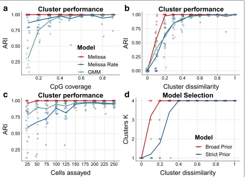
(i.e., cell sub-populations are difficult to distinguish), the performance drops; however, Melissa is consistently supe-rior to the Melissa Rate and GMM models and rapidly reaches near-perfect clustering accuracy. Similarly, when varying the total number of cells assayed in each exper-iment (see Fig. 3c), Melissa retains its almost perfect clustering performance and is still consistently superior than the competing models.

Subsequently, we test Melissa’s ability to perform model selection, that is, to identify the appropriate number of cell sub-populations. To do so, we run the model on sim-ulated data, setting the initial number of clusters toK = 10 and letting the variational optimization prune away inactive clusters [26]. We used both broad (red line) and shrinkage (blue line) priors. Figure3d shows that the vari-ational optimization automatically recovered the correct number of mixture components for almost all parame-ter settings. As expected, in settings with high between cluster similarity, the model with shrinkage prior returned fewer clusters, since the data complexity term in Eq. (9) (see the “Methods” section) was penalizing more the vari-ational approximation compared to the gain in likelihood from explaining the data. Finally, we assess the scalabil-ity of Melissa with respect to the number of single cells. Additional file1: Figure S3 compares the variational Bayes (red line) with the Gibbs sampling (blue line) algorithm, which demonstrates the good scalability of variational inference where we can analyze thousands of single cells in acceptable running times. The maximum number of

iterations for the variational Bayes algorithm was set to 400, and the Gibbs algorithm was run for 3000 iterations. Both algorithms are implemented in the R programming language and were run on a machine utilizing at most 16 CPU cores.

a

b

c

d

Fig. 3Melissa efficiently and accurately clusters cell sub-populations.aClustering performance measured by ARI as we vary CpG coverage. Higher values correspond to better agreement between predicted and true cluster assignments. For each CpG coverage setting, a total of 10 random splits of the data to training and test sets was performed. Each colored circle corresponds to a different simulation. The plot shows also the LOESS curve for each method as we increase CpG coverage.bClustering performance (ARI) for varying proportions of similar genomic regions between clusters. cClustering performance (ARI) as we vary the total number of cells assayed.dPredicted number of clusters using two different prior settings: a broad and a strict prior as we vary cluster dissimilarity. Initial number of clusters was set toK=10. Melissa identifies the correct number of clusters in most parameter settings (K=4); notably when there is no dissimilarity across clusters (i.e., we have one global cell sub-population), Melissa prunes away all components and keeps only one cluster (K=1)

0.5% of the mapped reads were sub-sampled to gener-ate pseudo-single-cell methylomes. Subsequently, reads falling in the same genomic site were binarised to obtain a digital output of methylation. Finally, the two cell lines were combined in a single data set of 80 pseudo-single cells prior to running Melissa. This procedure produces data with a more similar structure to real scBS-seq data, since the uneven read coverage better captures the struc-ture of missing data observed in single cell epigenomic experiments.

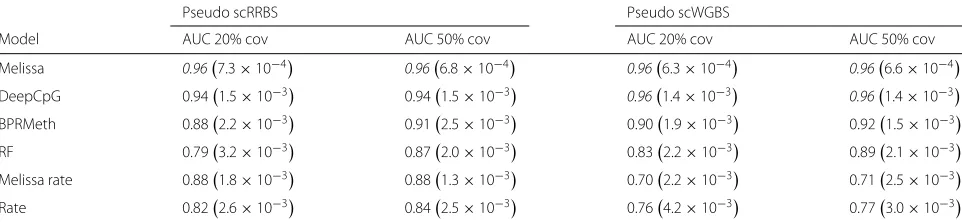
Table 1 shows the results for the two studies when imputing CpGs falling in genomic regions of ±2.5 kb around transcription start sites (TSS) for different levels of CpG coverage. Consistently with the simulation study in

Table 1Melissa robustly imputes CpG methylation states on sub-sampled ENCODE scRRBS and scWGBS synthetic data. Entries with italics denote the model with the highest performance in terms of AUC

Pseudo scRRBS Pseudo scWGBS

Model AUC 20% cov AUC 50% cov AUC 20% cov AUC 50% cov

Melissa 0.967.3_×10−4 _0.966.8×10−4 _0.966.3×10−4 _0.966.6×10−4

DeepCpG 0.941.5_×10−3 _0.941.5×10−3 _0.961.4×10−3 _0.961.4×10−3

BPRMeth 0.882.2×10−3 _0.912.5×10−3 _0.901.9×10−3 _0.921.5×10−3

RF 0.793.2×10−3 _0.872.0×10−3 _0.832.2×10−3 _0.892.1×10−3

Melissa rate 0.881.8×10−3 _0.881.3×10−3 _0.702.2×10−3 _0.712.5×10−3

Rate 0.822.6×10−3 _0.842.5×10−3 _0.764.2×10−3 _0.773.0×10−3

Imputation performance in terms of AUC as we vary the proportion of covered CpGs used for training. Higher values correspond to better imputation performance. For each CpG coverage setting, a total of 10 random splits of the data to training and test sets was performed; shown are the mean AUC value together with two standard deviations of the estimate in parenthesis. Note that DeepCpG was trained once on two chromosomes; hence, the values do not change as we vary the CpG coverage

file1: Figure S4–S9). Finally, Melissa could easily separate both cell sub-populations for all settings considered in this study.

Melissa accurately predicts methylation states on real data To assess Melissa’s performance on real scBS-seq data, we considered two mouse ESC data sets generated from scM&T-seq [11] and scBS-seq [8] protocols. The mouse ESCs were cultured either in 2i medium (2i ESCs) or serum conditions (serum ESCs); hence, we expect methy-lation heterogeneity between cell sub-popumethy-lations. In addition, in serum ESCs, there is evidence of additional CpG methylation heterogeneity [27], making these data suitable for the model selection task to infer cell sub-population structure. The analysis on both data sets was performed on six different genomic contexts: protein coding promoters with varying genomic windows:±1.5 kb, ±2.5 kb, and ±5 kb around TSS, active enhancers, super enhancers, and Nanog regulatory regions (see the “Methods” section for details on data preprocessing). It should be noted that DeepCpG is designed to predict individual missing CpGs, rather than missing regions, and requires always information about neighboring CpGs. This means that, during prediction,DeepCpGalways has access to more data than competing methods, potentially providing it with an unfair advantage; to partly address this problem, we also present results when DeepCpG had access to sub-sampled data (labeledDeepCpG Subin our figures). In general, DeepCpGshould be thought as complementary to Melissa, and comparisons should be evaluated cautiously (see below).

We first applied Melissa on the scM&T-seq data set which consists of 75 single cells (142i ESCsand 61serum ESCs). Figure4a shows a direct comparison of the impu-tation performance of all the methods across a variety of genomic contexts. Melissa is better or comparable to rival methods in terms of AUC (see Fig.4a) and substan-tially more accurate in terms of F-measure (Additional

file 1: Figure S10), demonstrating its ability to capture local CpG methylation patterns.DeepCpGalso performs strongly on most genomic regions, indicating that a flexi-ble deep learning method is effective in capturing patterns of methylation. Similar results were obtained by consider-ing different metrics (Additional file1: Figure S10–S12). Boxplots show performance distributions across 10 inde-pendent training/test splits of the data, except for Deep-CpG, where the high computational costs prevented such investigation. Interestingly, methods based on methyla-tion rates performed poorly at promoters, underlining the importance of methylation profiles in distinguishing epigenetic state near transcription start sites and iden-tifying meaningful cell sub-populations. For all models, the imputation performance (in terms of AUC) at active enhancers was lower, indicating high methylation vari-ability across cells and neighboring CpG sites as shown in [8].

a

b

Fig. 4Imputation performance and clustering of scM&T-seq mouse ESCs [11] based on genome wide methylation profiles.aPrediction performance on test set for imputing CpG methylation states in terms of AUC. Higher values correspond to better imputation performance. Each colored boxplot indicates the performance using 10 random splits of the data in training and test sets; due to high computational costs, DeepCpG was trained only once and the boxplots denote the variability across ten random sub-samplings of the test set.bExample promoter regions with the predicted methylation profiles for three developmental genes:Myc, Esrrb, andNog. Each colored profile corresponds to the average methylation pattern of the cells assigned to each sub-population, in our case Melissa identifiedK₌3 clusters

hypo-methylated CpG islands). Interestingly, 2i cells can be easily separated from serum cells based on methyla-tion rate alone, due to the global hypo-methylamethyla-tion of 2i cells; however, the sub-population structure within serum cells appears to be determined by changes in profiles.

As a second real data set, we analyzed the smaller scBS-seq data set which consists of only 32 cells (122i ESCsand 20serum ESCs). The imputation performance in terms of AUC across genomic contexts is shown in Fig.5. Melissa retains its high prediction accuracy and is comparable with DeepCpG across most contexts (see Additional file 1: Figure S14–S16 for performance on different metrics), even though the full DeepCpG model has slightly bet-ter performance on this data set. This suggests that the small number of cells in this data set did not allow an effective sharing of information. In terms of clustering

performance, Melissa identifies three clusters in the vast majority of settings, once again underlying the emergence of epigenomically distinct populations within serum cells (see Additional file 1: Figure S17 and S18 for example methylation profiles across genomic contexts).

A note on the comparison with DeepCpG

Fig. 5Imputation performance of scBS-seq mouse ESCs [8] based on genome-wide methylation profiles. Shown is the prediction performance, in terms of AUC, for imputing CpG methylation states. Each colored boxplot indicates the performance using 10 random splits of the data in training and test sets; due to high computational costs, DeepCpG was trained only once and the boxplots denote the variability across ten random sub-samplings of the test set

required around 3 to 4 days to analyze each data set on a GPU cluster equipped with high end NVIDIA Tesla K40ms GPUs, and had very high memory requirements. These computational overheads effectively make Deep-CpG out of reach for smaller research groups. On the other hand, Melissa operates on a set of genomic contexts of interest (e.g., promoters), while DeepCpG is designed for genome-wide imputation; computational performance of both methods will therefore depend on specific choices, such as the size/number of the regions of interest for Melissa, or the number of training chromosomes for DeepCpG.

In addition to the differences in scope between the two methods, one should also be cautious when directly comparing prediction performances due to the different design of the DeepCpG model. DeepCpG is trained on a specific set of chromosomes and considers each CpG site independently; hence, it does not have a notion of genomic region to be trained on and will in any case utilize information from neighboring CpGs within or outside the region, information that Melissa and the rival methods do not have access to.

Conclusions

Single-cell DNA methylation measurements are rapidly becoming a major tool to understand epigenetic gene reg-ulation in individual cells. Newer platforms are rapidly expanding the scope of the technology in terms of assaying large numbers of cells [14]; however, all technologies are plagued by intrinsically low coverage in terms of numbers of CpGs assayed.

In this paper, we have proposed Melissa as a way of addressing the low coverage issue by sharing information

between CpGs with a local smoothing and between cells with a Bayesian clustering prior. On both synthetic and real data, Melissa achieved state-of-the art imputation performance over a panel of competing methods, includ-ing DeepCpG [24] and random forests. While achiev-ing comparable or superior performance to black-box methods, such as neural networks and random forests, Melissa is more transparent and needs minimal tun-ing: all the results shown, on both synthetic and real data, were obtained with the same settings of the algo-rithm. Additionally, as all Bayesian methods, Melissa out-puts are probability distributions that fully quantify the uncertainty on the model’s prediction, and which are more easily usable for further experimental design compared to the point-estimates provided by black-box approaches. Melissa does not require additional annotation data as in [23] or [28] and does not exploit sequence information like DeepCpG, but an extension leveraging side data would be easily accomplished within the Bayesian framework and would represent an interesting extension for future research. By using a Bayesian clustering prior, Melissa has the added benefit of simultaneously uncovering the pop-ulation structure within the assay, as we demonstrated in the real data examples; Melissa can therefore be a useful tool in uncovering epigenetic diversity among cells.

methylomes using a Bayesian probabilistic model. Epiclo-mal shares a similar hierarchical structure to Melissa and also models bisulfite conversion error; however, Epiclomal does not model the spatial variability of neighboring CpGs and therefore cannot perform imputation as Melissa does. While Melissa accounts for heterogeneity in the cell population structure, it does not allow for heterogeneity at the single-gene level: each cluster has a single methy-lation profile within each region, and all variability at the single locus level is attributed to noise. This rigidity limits the usefulness of Melissa as a tool to investigate intrinsic stochasticity in methylation at the single locus level. Relaxing the modeling assumptions to accommo-date methylation variability in Melissa is an interesting topic for future research. Another area where Melissa could be fruitfully applied is the integrative study of mul-tiple high-throughput features in single cells. Recently, Kapourani and Sanguinetti [16] showed that features extracted from methylation profiles could be effectively used to predict gene expression in bulk experiments. With the advent of novel technologies measuring gene expres-sion and multiple epigenomic features in individual cells [13], interpretable Bayesian models like Melissa are likely to play an important role in furthering our understanding of epigenetic control of gene expression in single cells.

Methods Melissa model

In order to provide spatial smoothing of the methylation profiles at specific regions, we adapt a generalized linear model of basis function regression proposed recently [16] and further extended and implemented in the BPRMeth Bioconductor package [21]. The basic idea of BPRMeth is as follows: the methylation profile associated with a genomic regionmis defined as a (latent) functionf:m→

(0, 1)which takes as input the genomic coordinate along the region and returns the propensity for that locus to be methylated. For single-cell methylation data, methylation of individual CpG sites can be naturally modeled using a Bernoulli observation model, since for the majority of covered sites we have binary CpG methylation states (see Additional file1: Figure S13). More specifically, for a spe-cific regionm, we model the observed methylation of CpG siteias:

ymi∼Bern(ρmi), (1) where the unknown “true” methylation levelρmi has as covariates the CpG locations xmi. Then, we define the BPRMeth model as:

ηmi=wmh(xmi), fm(xmi)=ρmi=g−1(ηmi),

(2)

wherewm are the regression coefficients,xmi ≡ h(xmi) are the basis function transformed CpG locations (here we

consider radial basis functions (RBFs)), andg(·)is the link function that allows us to move from the systematic com-ponents ηmi to mean parametersρmi. Here we consider aprobit regression model which is obtained by defining g−1(·)=(·)— where(·)denotes the cdf of the standard normal distribution—ensuring thatf takes values in the [ 0, 1] interval. Notice that both BPRMeth and Melissa do not explicitly model bisulfite conversion errors. Conver-sion errors are estimated to be relatively rare and below 1% [30], and we show in our simulation studies that Melissa is highly robust to the addition of noise mimicking possible errors.

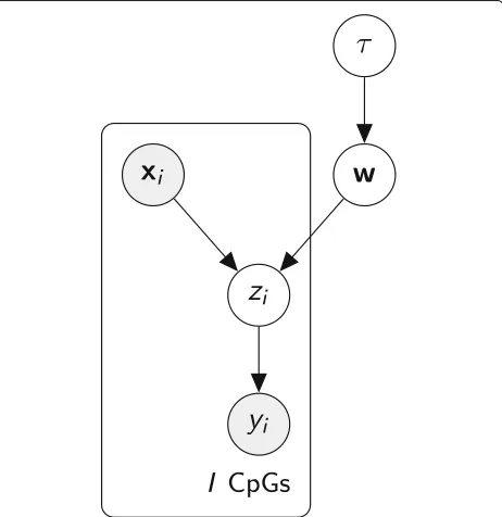
To account for the limited CpG coverage of scBS-seq experiments, the BPRMeth model was recently reformu-lated in a Bayesian framework [21]. The model was made amenable to Bayesian estimation thanks to a data augmen-tation strategy [31]. This strategy consists of introducing an additional auxiliary latent variablezi, which has a Gaus-sian distribution conditioned on the inputwxi, leading to the graphical model in Fig.6.

The BPRMeth model is limited to sharing informati.on across CpGs via local smoothing (which certainly helps in dealing with data sparsity); however, in our experience the coverage in scBS-seq data is insufficient to infer infor-mative methylation profiles at many genomic regions. We therefore propose Melissa to exploit the population struc-ture of the experimental design and additionally share and transfer information across cells.

Assume that we haveN(n=1, ...,N)cells and each cell consists ofM(m = 1, ...,M) genomic regions, for exam-ple promoters, and we are interested in both partitioning

the cells inK clusters and inferring the methylation pro-files for each genomic region. To do so, we use a finite Dirichlet mixture model (FDMM) [32], where we assume that the methylation profile of the mth region for each cellnis drawn from a mixture distribution withK com-ponents (where K < N). This way, cells belonging to the same cluster will share the same methylation profile, although profiles will still differ across genomic regions. Letcnbe a latent variable comprising a 1-of-K binary vec-tor with elementscnk representing the component that is responsible for celln, andπkbe the probability that a cell belongs to clusterk, i.e.πk =p(cnk =1). The conditional distribution ofC= {c1,. . .,cN}givenπis:

p(C|π)=

N

n=1

K

k=1 πcnk

k . (3)

Considering the FDMM as a generative model, the latent variables cn will generate the latent observations

Zn∈RM×Im, which in turn will generate the binary obser-vationsYn ∈ {0, 1}M×Im depending on the sign ofZn, as shown in Fig.6. The conditional distribution of the data (Z,Y), given the latent variables C and the component parametersW, becomes:

p(Y,Z|C,W,X)=

N

n=1 K

k=1

_M

m=1

p(ynm|znm)p(znm|wmk,Xnm) cnk

,

(4)

where

p(ynm|znm)=I(znm>0)ynmI(znm≤0)(111−ynm).

To complete the model, we introduce priors over the parameters. We choose a Dirichlet distribution over the mixing proportions,p(π) = Dir(π|δ0), where for sym-metry we choose the same parameterδ0k for each of the

mixture components. We also introduce an independent Gaussian prior over the coefficientsW, that is:

p(W|τ)=

M

m=1

K

k=1

N(wmk|0,τ_k−1I). (5)

Finally, we introduce a prior distribution for the (hyper)-parameter τ and assume that each cluster has its own precision parameter,p(τk) = Gamma(τk|α0,β0). Having defined our model, we can now write the joint distribution over the observed and latent variables:

p(Y,Z,C,W,π,τ|X)=p(Y|Z)p(Z|C,W,X)p(C|π)p(π)p(W|τ)p(τ), (6)

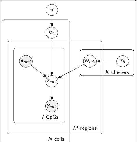
where the factorization corresponds to the probabilistic graphical model shown in Fig.7, resulting in the following hierarchical model:

π∼Dir(δ0) cn|π∼Discrete(π)

τk∼Gamma(α0,β0) wmk|τk∼N(0,τ_k−1I) znmi|wmk,xnmi∼N(w_mkxnmi, 1)

ynmi|znmi=

1 ifznmi>0 0 ifznmi≤0.

Importantly, Melissa is a hybrid between a global unsu-pervised clustering model and a local suunsu-pervised pre-diction model, encoded through the GLM regression coefficientswfor each genomic region. When consider-ing Melissa as an imputation (or predictive) model, the training data are coming by using only a subset of CpG tuples(xnmi,ynmi)for each region. For example, from the observedInmCpGs in a given region, Melissa will only see Inm/2 random CpGs during training, and the remaining CpGs will be used as a held out test set to evaluate its pre-diction performance. Note that in any case, either using all CpGs or a subset during training, Melissa will addition-ally perform clustering at the global level which is encoded through the latent variablescn.

Variational inference

The posterior distribution of the latent variables given the observed datap(Z,C,W,π,τ|Y,X)for the Melissa model is not analytically tractable; hence, we resort to approxi-mate techniques. The most common method for approx-imate Bayesian inference is to perform Markov Chain Monte Carlo (MCMC) [33]; however, sampling meth-ods require considerable computational resources and do not scale well when performing genome-wide analysis on hundreds or thousands of single cells. Variational meth-ods can provide an efficient, approximate solution with better scalability in this case (see the “Results” section for a comparison between Gibbs sampling and varia-tional inference for this model). More specifically, we use mean-field variational inference [34] which assumes that the approximating distribution factorizes over the latent variables:

q(Z,C,W,π,τ)=q(Z)q(C)q(W)q(π)q(τ). (7) Detailed mathematical derivations of the optimal varia-tional factors are available in Addivaria-tional file1: Section 1. Next, we iteratively update each factorqwhile holding the remaining factors fixed using the coordinate ascent vari-ational inference (CAVI) algorithm which is summarized in Algorithm1.

Predictive density and model selection

Given an approximate posterior distribution, we are in the position to predict the methylation level at unobserved CpG sites. The predictive density of a new observation y∗, which is associated with latent variables c∗, z∗ and covariatesX∗, is given by:

p(y_∗|X_∗,Y)= c∗

p(y_∗,c_∗,z_∗,θ|X_∗,Y)dθdz_∗

K

k=1

δk

jδjB

ern ⎛ ⎜ ⎝y∗

⎛ ⎜

⎝ X∗λk I+diagX_∗SkXT∗

⎞ ⎟ ⎠ ⎞ ⎟ ⎠

(8)

where we collectively denote asθthe relevant parameters being marginalized.

It has been repeatedly observed [26] that, when fit-ting variationally a mixture model with a large number of components, the variational procedure will prune away components with no support in the data, hence effec-tively determining an appropriate number of clusters in an automatic fashion, i.e., perform model selection. We can gain some intuition as to why this happens in the following way. We can rewrite the Kullback-Leibler (KL) divergence as:

KL(q(θ)||p(θ|X))=lnp(X)−lnp(X|θ)_q(θ)+KL(q(θ)||p(θ)) (9)

where lnp(X) can be ignored since it is constant with respect to q(θ). To minimize this objective function, the variational approximation will both try to increase the expected log likelihood of the data lnp(X|θ) while minimizing its KL divergence with the prior distribu-tion p(θ). Hence, using variational Bayes, we have an automatic trade-off between fitting the data and model complexity [19].

Assessing Melissa via a simulation study

To generate realistic simulated single-cell methylation data, we first used the BPRMeth package [21] to infer five prototypical methylation profiles from the GM12878 lymphoblastoid cell line. The bulk BS-seq data for the GM12878 cell line are publicly available from the ENCODE project [35]. Based on these profiles, we simulated single-cell methylation data (i.e., binary CpG methylation states) forM= 100 genomic regions, where each CpG was generated by sampling from a Bernoulli dis-tribution with probability of success given by the latent function evaluation at the specific site. To mimic the inherent noise introduced by bisulfite conversion error, Gaussian noiseN(μ = 0,σ = 0.05) was introduced to the probability of success prior to generating each binary CpG site. This process can be thought of as generat-ing methylation data for a specific sgenerat-ingle cell. Next, we generatedK = 4 cell sub-populations by randomly shuf-fling the genomic regions across clusters, so now each cell sub-population has its own methylome landscape. In total, we generated N = 200 cells, with the following cell sub-population proportions: 40%, 25%, 20%, and 15%. Additionally, to account for different levels of similarity between cell sub-populations, we simulated 11 different data sets by varying the proportion of similar genomic regions between clusters. Finally, to assess the perfor-mance of Melissa for varying number of cells assayed, we simulated 10 different data sets by varying the total number of single cells N. The scripts (written in the R pro-gramming language) for this simulation study are publicly available on the Melissa repository.

Algorithm 1CAVI for Melissa model

1: initializeGaussian factorλ,S; Dirichlet factorδ0; and Gamma factorα0,β0.

2: Updateαk ←α0+MD/2 3: Updateβk ←β0

4: whileELBO has not convergeddo

5: Setγnmk =(znm−Xnmwmk) Variational E-step 6: Updaternk∝ lnπkq(πk)+

m

−1

2γnmk γnmk

q(znm,wmk)

7: Variational M-step

8: Updateδk ←δ0k+

nrnk Dirichlet distribution parameter

9: Updateβ_k ←β0+1₂m

w_mkwmk

q(wmk) Gamma distribution parameter

10: Updateμnmi←krnk

w_mkxnmi

q(wmk) Mean of truncated Gaussian

11: Setznmiq(znmi)=

μnmi+φ(−μnmi)/

1−(−μnmi)

ifynmi=1

μnmi−φ(−μnmi)/(−μnmi) ifynmi=0 12: UpdateSmk ←

αk βkI+

nrnkXnmXnm

−1

Regression coefficient covariance 13: Updateλmk ←Smk

nrnkXnmznmq(znm) Regression coefficient mean

14: UpdateL(q(W,Z,C,π,τ)) Compute ELBO

15: end while

human genome; however, they require high-sequencing depth to obtain an accurate estimate of the bulk methy-lation level at each CpG site. To retain the structure of missing data observed in scBS-seq experiments (due to read length), we directly sub-sampled the raw FASTQ files which essentially lead to discarding individual reads rather than individual CpGs. For the RRBS data set, from each cell line, we generated 40 pseudo-single cells by randomly keeping 10% of the mapped reads from the bulk experi-ment, resulting in 80 cells when combining both cell lines. For the WGBS data set, the same number of pseudo-single cells was generated from each cell line, with the only dif-ference that only 0.5% of the mapped reads were retained from the bulk data due to the high-sequencing depth of the experiments. This process was performed for chro-mosomes 1 to 6 to alleviate the computational burden. Subsequently, the same preprocessing steps detailed in the previous section were performed, with the only difference that for this study we considered only±2.5 kb and±5 kb promoter regions around TSS. Each model, except Deep-CpG, used 20%, 50%, and 80% of the CpGs as training set, and the remaining of CpGs were used as a test set to eval-uate imputation performance. The DeepCpG model used chromosomes 1 and 3 as training set, chromosome 5 as validation set, and the remaining chromosomes as test set.

scBS-seq data and preprocessing

Single-cell bisulfite sequencing protocols provide us with single base-pair resolution of CpG methylation states. Since we assay the DNA of a single cell, the methylation

level for each CpG site is predominantly binary, either methylated or unmethylated. However, due to each chromosome having two copies, a small proportion of CpG sites have a non-binary nature (see Additional file1: Figure S19). To avoid ambiguities, hemi-methylated sites—sites with 50% methylation level—are filtered prior to downstream analysis, and for the remaining sites, binary methylation states are obtained from the ratio of methylated read counts to total read counts [11].

Since Melissa considers genomic regions for a specific genomic context, we use the BPRMeth package [21] to fil-ter CpGs that do not fall inside these regions, and create a simple data structure where each cell is a encoded as a list, and each entry of the list—corresponding to a spe-cific genomic region—is a matrix with two columns: the (relative) CpG location and the methylation state. We con-sidered six different genomic contexts where we applied Melissa: protein coding promoters with varying genomic windows:±1.5 kb,±2.5 kb, and±5 kb around transcrip-tion start sites (TSS), active enhancers, super enhancers, and Nanog regulatory regions. Due to the sparse CpG cov-erage, for the three genomic contexts except promoters, we filtered loci with smaller than 1 kb annotation length, and specifically for Nanog regions, we took a window of

±2.5 kb around the center of the genomic annotation. In addition, we only considered regions that were covered in at least 50% of the cells with a minimum coverage of 10 CpGs and had between cell variability; the ratio-nale being that homogeneous regions across cells do not provide additional information for identifying cell sub-populations. The CpG coverage distribution after the fil-tering process across different genomic contexts is shown in Additional file1: Figure S20 and S21. The sparsity level of the two scBS-seq data sets across different genomic contexts is shown in Additional file1: Table S3. It should be noted that imputation performance is evaluated only on genomic regions that pass the filtering threshold. We run the model withK = 6 andK = 5 clusters for the scM&T-seq and scBS-seq data sets, respectively, and we use a broad prior over the model parameters.

Performance evaluation

To assess model performance across all genomic contexts, we partition the data and use 50% of the CpGs in each cell and region for training set and the remaining 50% as test set (except DeepCpG, see below). The prediction per-formance of all competing models, except DeepCpG, was evaluated on imputing all missing CpG states in a given region at once. For computing binary evaluation metrics, such asF-measure, predicted probabilities above 0.5 were set to one and rounded to zero otherwise.

F-measure TheF-measure orF1-score is the harmonic mean of precision and recall:

F-measure=2· precision·recall

precision+recall. (10)

Gaussian mixture model The input to the Gaussian mixture model (GMM) is the average methylation rate across the region; since rates are between (0,1), we transform them to M values, which follow closer the

Gaussian distribution [22]. The transformation from aver-age methylation rates to averaver-ageMvalues is obtained by:

Mvalue=log₂

rate+0.01 1−rate+0.01

. (11)

Adjusted Rand Index The Adjusted Rand Index (ARI) is a measure of the similarity between two data clusterings:

ARI= ij _nij 2

−i

_αi 2 j

_βj 2

/n

2 1 2 i _αi 2

+j

βj 2

−i

_αi 2 j

βj 2

/n

2 .

(12)

DeepCpG

The DeepCpG method takes a different imputation approach: it is trained on a specific set of chromosomes and predicts methylation states on the remaining chro-mosomes where it imputes each CpG site sequentially by using as input a set of neighboring CpG sites. This approach makes it difficult to equally compare with the rival methods, since for each CpG the input features to DeepCpG are all the neighboring sites, whereas the com-peting models have access to a subset of the data and they make predictions in one pass for the whole region. Since we only had access to CpG methylation data and to make it comparable with the considered methods, we trained the CpG module of DeepCpG (termedDeepCpG CpGin [24]). For the scM&T-seq data set, chromosomes 3 and 17 were used as training set, chromosomes 12 and 14 as vali-dation set and the remaining chromosomes as test set. For the scBS-seq data set, chromosomes 3, 17, and 19 were used as training set; chromosomes 12 and 14 as validation set; and the remaining chromosomes as test set. The cho-sen chromosomes had at least three million CpGs used as training set, a sensible size for the DeepCpG model as suggested by the authors. A neighborhood ofK= 20 CpG sites to the left and the right for each target CpG was used as input to the model. During testing time, even if a given genomic region did not contain at least 40 CpGs, the DeepCpG model used additional CpGs outside this window to predict methylation states, hence using more information compared to the rival models. In total, the DeepCpG model took around 4 days per data set for train-ing and prediction on a cluster equipped with NVIDIA Tesla K40ms GPUs.

Additional file

Abbreviations

ARI: Adjusted Rand Index; AUC: Area under the receiver operating

characteristic curve; BPRMeth: Bayesian probit regression for methylation; bp: Base pair; CAVI: Coordinate ascent variational inference; CPU: Central processing unit; ESC: Embryonic stem cell; GEO: Gene expression omnibus; GLM: Generalized linear model; GMM: Gaussian mixture model; GPU: Graphics processing unit; MCMC: Markov chain Monte Carlo; RBF: Radial basis function; RF: Random Forest; scBS-seq: Single-cell bisulfite sequencing; scRRBS: Single-cell reduced representation bisulfite sequencing; TSS: Transcription start site; WGBS: Whole genome bisulfite sequencing

Acknowledgements

We thank Duncan Sproul and Jon Higham for discussion and help with bioinformatics pipeline analysis and Oliver Stegle, Michalis Michaelides, Ricard Argelaguet, and Stephen Clark for valuable comments and discussion.

Funding

CAK is a cross-disciplinary post-doctoral fellow supported by funding from the University of Edinburgh, Medical Research Council (core grant to the MRC Institute of Genetics and Molecular Medicine), and the EPSRC Centre for Doctoral Training in Data Science, funded by the UK Engineering and Physical Sciences Research Council (grant EP/L016427/1).

Availability of data and materials

The Melissa model is publicly available as R software released under the GNU GPL-3 licence (Github:https://github.com/andreaskapou/Melissa[37], Bioconductor:http://bioconductor.org/packages/Melissa/[38], and DOI: https://dx.doi.org/10.5281/zenodo.2567427). The scBS-seq data from mouse ESCs from [8] are available under GEO accession number GSE56879. The scM&T-seq data from mouse ESCs from [11] are available under GEO accession number GSE74535.

Authors’ contributions

Both authors conceived the study, carried out the data analysis, and wrote the paper. CAK implemented and evaluated the method. Both authors read and approved the final manuscript.

Ethics approval and consent to participate

Ethical approval was not needed for this study.

Consent for publication

Not applicable.

Competing interests

The authors declare that they have no competing interests.

Publisher’s Note

Springer Nature remains neutral with regard to jurisdictional claims in published maps and institutional affiliations.

Author details

1_{School of Informatics, University of Edinburgh, Edinburgh EH8 9AB, UK.}2_MRC

Institute of Genetics and Molecular Medicine, University of Edinburgh, Edinburgh EH4 2XU, UK.3_{Synthetic and Systems Biology, University of} Edinburgh, Edinburgh EH9 3BF, UK.

Received: 5 October 2018 Accepted: 28 February 2019

References

1. Bird A. DNA methylation patterns and epigenetic memory. Genes Dev. 2002;16(1):6–21. Available from:http://www.ncbi.nlm.nih.gov/pubmed/ 11782440.

2. Baylin SB, Jones Pa. A decade of exploring the cancer epigenome -biological and translational implications. Nat Rev Cancer. 2011;11(10): 726–34. Available from:http://dx.doi.org/10.1038/nrc3130.

3. Jones PA. Functions of DNA methylation: islands, start sites, gene bodies and beyond. Nat Rev Genet. 2012;13(7):484–92. Available from:http:// www.ncbi.nlm.nih.gov/pubmed/22641018.

4. Krueger F, Kreck B, Franke A, Andrews SR. DNA methylome analysis using short bisulfite sequencing data. Nat Methods. 2012;9(2):145–51. Available from:http://www.ncbi.nlm.nih.gov/pubmed/22290186. 5. Shapiro E, Biezuner T, Linnarsson S. Single-cell sequencing-based

technologies will revolutionize whole-organism science. Nat Rev Genet. 2013;14(9):618–30. Available from:http://www.ncbi.nlm.nih.gov/ pubmed/23897237.

6. Schwartzman O, Tanay A. Single-cell epigenomics: techniques and emerging applications. Nat Rev Genet. 2015;16(12):716–26. Available from:http://dx.doi.org/10.1038/nrg3980.

7. Kelsey G, Stegle O, Reik W. Single-cell epigenomics: Recording the past and predicting the future. Science. 2017;358(6359):69–75. Available from: http://dx.doi.org/10.1017/S0022215115001383.

8. Smallwood Sa, Lee HJ, Angermueller C, Krueger F, Saadeh H, Peat J, et al. Single-cell genome-wide bisulfite sequencing for assessing epigenetic heterogeneity. Nat Methods. 2014;11(8):817–20. Available from:http:// www.ncbi.nlm.nih.gov/pubmed/25042786.

9. Guo H, Zhu P, Wu X, Li X, Wen L, Tang F. Single-cell methylome landscapes of mouse embryonic stem cells and early embryos analyzed using reduced representation bisulfite sequencing. Genome Res. 20132126–35. Available from:http://www.ncbi.nlm.nih.gov/pubmed/ 24179143.

10. Farlik M, Sheffield NC, Nuzzo A, Datlinger P, Schönegger A, Klughammer J, et al. Single-Cell DNA Methylome Sequencing and Bioinformatic Inference of Epigenomic Cell-State Dynamics. Cell Rep. 2015;10(8):1386–97. Available from:http://www.ncbi.nlm.nih.gov/ pubmed/25732828.

11. Angermueller C, Clark SJ, Lee HJ, Macaulay IC, Teng MJ, Hu TX, et al. Parallel single-cell sequencing links transcriptional and epigenetic heterogeneity. Nat Methods. 2016;13(3):229–32. Available from:http:// www.ncbi.nlm.nih.gov/pubmed/26752769.

12. Hou Y, Guo H, Cao C, Li X, Hu B, Zhu P, et al. Single-cell triple omics sequencing reveals genetic, epigenetic, and transcriptomic

heterogeneity in hepatocellular carcinomas. Cell Res. 2016;26(3):304–19. Available from:http://www.ncbi.nlm.nih.gov/pubmed/26902283. 13. Clark SJ, Argelaguet R, Kapourani CA, Stubbs TM, Lee HJ, Alda-Catalinas

C, et al. ScNMT-seq enables joint profiling of chromatin accessibility DNA methylation and transcription in single cells. Nat Commun. 2018;9(1):1–9. Available from:http://dx.doi.org/10.1038/s41467-018-03149-4.http:// www.ncbi.nlm.nih.gov/pubmed/29472610.

14. Luo C, Keown CL, Kurihara L, Zhou J, He Y, Li J, et al. Single-cell methylomes identify neuronal subtypes and regulatory elements in mammalian cortex. Science. 2017;357(6351):600–4. Available from:http:// www.ncbi.nlm.nih.gov/pubmed/28798132.

15. Mulqueen RM, Pokholok D, Norberg SJ, Torkenczy KA, Fields AJ, Sun D, et al. Highly scalable generation of DNA methylation profiles in single cells. Nat Biotechnol. 2018;36(5):428–31. Available from:http://www.ncbi. nlm.nih.gov/pubmed/29644997.

16. Kapourani CA, Sanguinetti G. Higher order methylation features for clustering and prediction in epigenomic studies. Bioinformatics. 2016;32(17):i405–12. Available from:http://www.ncbi.nlm.nih.gov/ pubmed/27587656.http://dx.doi.org/10.1093/bioinformatics/btw432. 17. Mayo TR, Schweikert G, Sanguinetti G. M 3 D: A kernel-based test for

spatially correlated changes in methylation profiles. Bioinformatics. 2015;31(6):809–16. Available from:http://www.ncbi.nlm.nih.gov/ pubmed/25398611.

18. Vanderkraats ND, Hiken JF, Decker KF, Edwards JR. Discovering high-resolution patterns of differential DNA methylation that correlate with gene expression changes. Nucleic Acids Research. 2013;41(14):6816–6827. Available from:http://www.ncbi.nlm.nih.gov/pubmed/23748561. 19. Bishop CM. Pattern recognition and machine learning: Springer; 2006.

Available from:http://www.library.wisc.edu/selectedtocs/bg0137.pdf. 20. Powers DMW. Evaluation: From Precision, Recall and F-Measure to ROC,

Informedness, Markedness & Correlation. J Mach Learn Technol. 2011;2(1): 37–63. Available from:http://dx.doi.org/10.1.1.214.9232.

21. Kapourani CA, Sanguinetti G. BPRMeth: a flexible Bioconductor package for modelling methylation profiles. Bioinformatics (Oxford, England). 2018;34(14):2485–6. Available from:http://www.ncbi.nlm.nih.gov/ pubmed/27587656.http://dx.doi.org/10.1093/bioinformatics/bty129. 22. Du P, Zhang X, Huang CC, Jafari N, Kibbe WA, Hou L, et al. Comparison

microarray analysis. BMC Bioinformatics. 2010;11(1):587. Available from: http://www.ncbi.nlm.nih.gov/pubmed/21118553.

23. Zhang W, Spector TD, Deloukas P, Bell JT, Engelhardt BE. Predicting genome-wide DNA methylation using methylation marks, genomic position, and DNA regulatory elements. Genome Biol. 2015;16(1):14. Available from:http://www.ncbi.nlm.nih.gov/pubmed/25616342. 24. Angermueller C, Lee HJ, Reik W, Stegle O. DeepCpG: accurate prediction

of single-cell DNA methylation states using deep learning. Genome Biol. 2017;18(1):67. Available from:http://www.ncbi.nlm.nih.gov/pubmed/ 28395661.

25. Hubert L, Arabie P. Comparing partitions. J Classif. 1985;2(1):193–218. Available from:http://dx.doi.org/10.1007/BF01908075.

26. Corduneanu A, Bishop CM. Variational Bayesian Model Selection for Mixture Distributions. In: In Artificial Intelligence and Statistics; 2001. p. 27–34. Available from:http://dx.doi.org/10.1016/j.csda.2006.07.020. 27. Ficz G, Hore TA, Santos F, Lee HJ, Dean W, Arand J, et al. FGF signaling

inhibition in ESCs drives rapid genome-wide demethylation to the epigenetic ground state of pluripotency. Cell Stem Cell. 2013;13(3):351–9. Available from:http://www.ncbi.nlm.nih.gov/pubmed/23850245. 28. Ernst J, Kellis M. Large-scale imputation of epigenomic datasets for

systematic annotation of diverse human tissues. Nat Biotechnol. 2015;33(4):364–76. Available from:http://dx.doi.org/10.1038/nbt.3157. 29. de Souza CPE, Andronescu M, Masud T, Kabeer F, Biele J, Laks E, et al.

Epiclomal: probabilistic clustering of sparse single-cell DNA methylation data. bioRxiv. 2018;414482.

30. Genereux DP, Johnson WC, Burden AF, Stöger R, Laird CD. Errors in the bisulfite conversion of DNA: modulating inappropriate-and

failed-conversion frequencies. Nucleic Acids Res. 2008;36(22):e150. Available from:http://www.ncbi.nlm.nih.gov/pubmed/18984622. 31. Albert JH, Chib S. Bayesian Analysis of Binary and Polychotomous

Response Data. J Am Stat Assoc. 1993;88(422):669–79. Available from: http://dx.doi.org/10.2307/2290350.

32. McLachlan G, Peel D. Finite mixture models. New York: Wiley; 2004. https://doi.org/10.1002/0471721182.

33. Gelfand A, Smith AFM. Sampling-Based Approaches to Calculating Marginal Densities. J Am Stat Assoc. 1990;85(410):398–409. Available from:http://dx.doi.org/10.2307/2289776.

34. Blei DM, Kucukelbir A, McAuliffe JD. Variational Inference: A Review for Statisticians. J Am Stat Assoc. 2017;112(518):859–77. Available from: http://dx.doi.org/10.1080/01X00000.621459.2017.1285773. 35. Dunham I, Kundaje A. Encode Project Consortium. An integrated

encyclopedia of DNA elements in the human genome. Nature. 2012;489(7414):57–74. Available from:http://www.ncbi.nlm.nih.gov/ pubmed/22955616.

36. Krueger F, Andrews SR. Bismark: A flexible aligner and methylation caller for Bisulfite-Seq applications. Bioinformatics. 2011;27(11):1571–2. Available from:http://www.ncbi.nlm.nih.gov/pubmed/21493656. 37. Kapourani CA, Sanguinetti G. Melissa: Bayesian clustering and imputation

of single cell methylomes. Github repository:,https://github.com/ andreaskapou/Melissa. 2019. Available from:https://dx.doi.org/10.5281/ zenodo.2567427.