A benchmark for RNA seq quantification pipelines

M E T H O D

Open Access

A benchmark for RNA-seq quantification

pipelines

Mingxiang Teng

, Michael I. Love

, Carrie A. Davis

, Sarah Djebali

, Alexander Dobin

, Brenton R. Graveley

,

Sheng Li

, Christopher E. Mason

, Sara Olson

, Dmitri Pervouchine

, Cricket A. Sloan

, Xintao Wei

, Lijun Zhan

and Rafael A. Irizarry

Abstract

Obtaining RNA-seq measurements involves a complex data analytical process with a large number of competing algorithms as options. There is much debate about which of these methods provides the best approach. Unfortunately, it is currently difficult to evaluate their performance due in part to a lack of sensitive assessment metrics. We present a series of statistical summaries and plots to evaluate the performance in terms of specificity and sensitivity, available as a R/Bioconductor package (http://bioconductor.org/packages/rnaseqcomp). Using two independent datasets, we assessed seven competing pipelines. Performance was generally poor, with two methods clearly underperforming and RSEM slightly outperforming the rest.

Background

RNA sequencing (RNA-seq) has become one of the most widely used technologies in biomedical research for highly parallel measurements of transcript expres-sion. For example, the ENCODE project is currently using RNA-seq to characterize the transcriptome of the project’s selection of cell lines [1]. The first step in quan-tifying transcription levels with RNA-seq is aligning reads, or pseudo-aligning parts of the read [2, 3], to transcripts. In this step, transcripts are either estimated from the data (de novo assembly) or predetermined from an existing database. In a second step, the expres-sion level for each of the transcripts in consideration is quantified for each sample. The algorithms considered here quantify expression for alternative transcripts within each gene and these can be combined to provide a summary for genes. We will refer to these two outputs astranscript levelandgene level, respectively.

Currently, there are several competing algorithms for both of these steps. In general, when a new method is published, authors typically claim superiority over exist-ing methods. This results in contradictory information

for those deciding on a method. This apparent contra-diction is due to the lack of a predetermined standard for comparison, which gives authors the freedom to se-lect evaluation procedures that favor their method. This phenomenon is known as the self-assessment trap [4]. To avoid this, one can define metrics beforehand that evaluate specificity/precision and sensitivity/accuracy. A previous study [5] implemented such an approach and evaluated 11 algorithms. All algorithms were found to perform remarkably well and none were reported to out-perform or underout-perform. However, accuracy assess-ments were related to the quantification of absolute expression levels, yet most RNA-seq studies are inter-ested in relative measures, or differential expression. Furthermore, the specificity assessment was based on the correlation of measurements from replicated experi-ments, a summary that we show to be suboptimal. Finally, most of the assessment was based on computer-simulated data that do not mimic experimental data in sources of variation, such as batch effects [6]. Here we contribute a new set of interpretable assessment metrics, motivated by previous work [7–9], that (1) relate to dif-ferential expression, (2) provide improvements over the use of correlation by considering direct estimates of variance, and (3) are based on data that better emulate experimental data. This set of assessments better dis-cerns the differences between the competing algorithms.

* Correspondence:[email protected] 1

Department of Biostatistics and Computational Biology, Dana-Farber Cancer Institute, 450 Brookline Avenue, Boston, MA 02215, USA

2_{Department of Biostatistics, Harvard TH Chan School of Public Health, 677} Huntington Avenue, Boston, MA 02115, USA

Full list of author information is available at the end of the article

© 2016 Teng et al.Open AccessThis article is distributed under the terms of the Creative Commons Attribution 4.0 International License (http://creativecommons.org/licenses/by/4.0/), which permits unrestricted use, distribution, and reproduction in any medium, provided you give appropriate credit to the original author(s) and the source, provide a link to the Creative Commons license, and indicate if changes were made. The Creative Commons Public Domain Dedication waiver (http://creativecommons.org/publicdomain/zero/1.0/) applies to the data made available in this article, unless otherwise stated. Tenget al. Genome Biology (2016) 17:74

To demonstrate the utility of our assessment metrics, we use them to compare the STAR [10], TopHat2 [11], and Bowtie2 [12] mapping methods and the Cufflinks [13], eXpress [14], Flux Capacitor [15], kal-listo [2], RSEM [16], Sailfish [3], and Salmon [17] quantification methods. We also developed a webtool (http://rafalab.rc.fas.harvard.edu/rnaseqbenchmark) that permits users to submit other competing methods.

Results Datasets

A key aspect of our proposed assessment is the availabil-ity of two datasets that permit the computation of the metrics. They are characterized by including two popula-tions, at least two replicates for each population, and a way to define beforehand which genes or transcripts are differentially expressed and which are not. The replicates permit the assessment of precision and comparing the two populations permits the assessment of sensitivity or the ability to discover real biological differences. Note that sensitivity is harder to assess because we need to know beforehand what differences to expect. In the past, this has been achieved with spike-in experiments [18–20]. However, the use of spike-ins has been criticized for not properly mimicking real experimental data [21].

The first represents the minimal dataset that can be used for the comparison. It includes two replicates for the cell lines GM12878 and K562. We used results from a microarray experiment comparing the same two cell lines to define real biological differences. We defined genes with a q-value smaller than 0.05 [22, 23] and abso-lute log fold changes larger than 1 as truly differentially expressed. Genes with q-values larger than 0.5 were de-noted as not differentially expressed. Genes in neither of these two groups were considered to be in a “grey area” and left out of the analysis. Note that we are not consid-ering microarrays to be a gold standard, but because the microarray data represents an independent measure-ment, algorithms that perform better at detecting real differences should, on average, show improved agree-ment with these independent results.

The second dataset was created using 30 samples from the Geuvadis project [24]. These samples were selected to represent a random sample of individuals. To intro-duce batch effect-like variability, we selected 15 from one center and 15 from another. These were then ran-domly divided into two groups both having seven sam-ples from one center and eight from another. Because the samples were assigned at random, this is a null ex-periment and we can consider the 15 samples in each group to be replicates. To distinguish the two groups, we used computer simulations to generate 2424 tran-scripts designed to be differentially expressed between the two groups. To make these abundances mimic

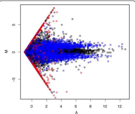
experimental data, we adapted the Polyester method [25] to include GC bias imitating the bias observed in the actual data. The resulting dataset mimics a real one quite well (Fig. 1).

The raw sequencing files for both datasets are available from the webtool (http://rafalab.rc.fas.harvard.edu/rnaseq-benchmark). Further details about both datasets are avail-able in the“Methods”section.

Calibration using control genes

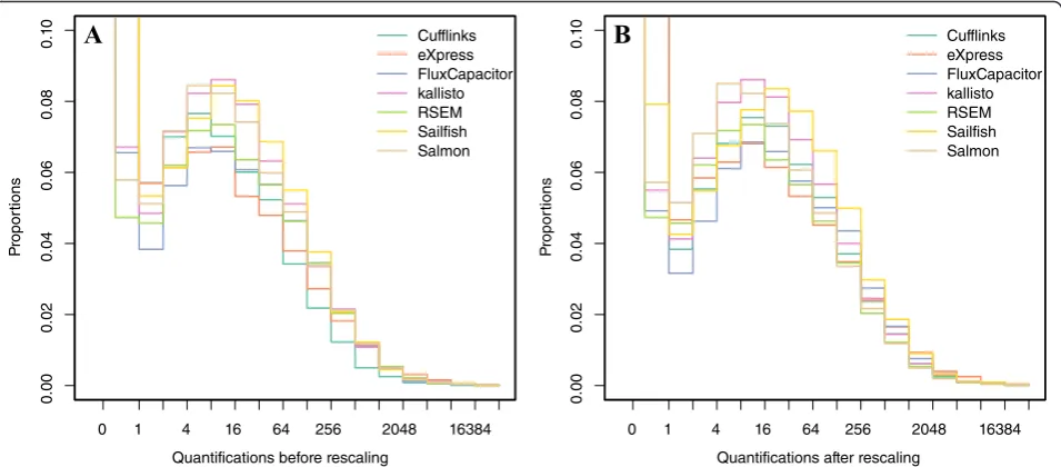
The first challenge to comparing performance across the different approaches is the lack of a standard unit for transcript level quantification. For example, Cufflinks reports fragments per kilobase of exon per million frag-ments mapped (FPKM); Flux Capacitor reports reads per kilobase of exon per million reads mapped (RPKM); eXpress, RSEM, Sailfish, kallisto, and Salmon report transcripts per million (TPM). Note that some of these algorithms provide options for what unit to return and we allowed each laboratory to decide which unit to re-port. Other analytical choices, such as the choice of normalization approach, add even more variability to the scales of the reported measures (Fig. 2a). The standard solutions to rescaling—for example, dividing by the median—are not appropriate because the median value for a typical sample is 0. Taking the median of the posi-tive values is not appropriate as it may introduce a bias in favor of or against methods that over- or underesti-mate the number of features with no expression. To

Fig. 1Estimated log fold changes stratified by transcript abundance on simulation dataset. One example based on Cufflinks quantification of two samples is shown here.Black pointsare non-differential transcripts;

blue pointsare differentially expressed transcripts which were simulated to have signals on both samples;red pointsare differentially expressed transcripts which were simulated to have signals in only one of the samples

overcome these challenges we considered only genes re-ported to be house-keeping genes [26], which are more likely to be expressed. Specifically, considering only this subset of genes for each algorithm, we compute the me-dian. Because house-keeping genes are typically expressed, this median value will not be 0. We then select one of the algorithms to serve as a reference baseline (we used RSEM, which reported in TPM) and we rescale all methods in the log-scale so that a value of 0 in the log-scale maps to a TPM of 1. Figure 2 shows the data before and after this re-scaling. Note that this is not meant as a normalization step, but rather as a simple rescaling so that the reported quanti-fications are approximately in the same units for all methods. Furthermore, note that fold change values are not affected by this re-scaling since the measurements for each algorithm are divided by the same constant which is cancelled out in fold-change calculations.

Correlation is not a measure of precision or reproducibility

The use of correlation to summarize reproducibility has become widespread in genomics [18, 27, 28]. Despite its English language definition, mathematically, correlation is not necessarily informative with regards to reproduci-bility. For this reason, we dedicate a subsection to ex-plain the major problems with this metric (details are provided in the“Methods”section).

The most egregious related mistake is to compute cor-relations of raw FPKM, RPKM, or TPM data. Averages, standard deviations, and correlations are popular sum-mary statistics for two-dimensional data because, for the bivariate normal distribution, these five parameters fully

describe the distribution [29]. However, RNA-seq data are not well approximated by bivariate normal data (Fig. 2). In fact, these data have a very large right tail, which implies that the correlation estimate can be highly susceptible to one point (Additional file 1: Figure S1a). Using the log transformation is a way to ameliorate this problem.

The standard way to quantify reproducibility between two sets of replicated measurements, say X1… XN and Y1… YN, is simply to determine how close they are to

each other. To quantify distance, we compute the math-ematical distance between them:

ffiffiffiffiffiffiffiffiffiffiffiffiffiffiffiffiffi ΣN

i¼1 d2i;

q

with di¼Xi−Yi

This metric decreases as reproducibility improves and is 0 when the reproducibility is perfect.

Another limitation with correlation is that it is defined from two lists and there is no standard way of applying it when more than one replicate is available. A standard measure of precision, the standard deviation (SD) across replicates, is more appropriate. Note that there is a con-nection between this metric and distance since the SD for two replicates is:

ffiffiffiffiffiffiffiffiffiffiffiffiffiffiffiffiffiffiffiffiffiffiffiffiffiffiffiffiffiffiffiffiffiffiffiffiffiffiffiffiffiffiffiffiffiffiffiffiffiffiffiffiffiffiffiffiffiffiffiffiffiffiffiffiffiffiffiffiffiffiffiffiffiffiffiffiffiffiffiffiffiffiffiffiffiffiffiffiffiffiffiffiffiffiffiffiffiffiffiffiffiffi 1

2 Xi −

Xi þ Yi 2

2

þ Yi −

Xi þ Yi 2

2

( )

s

¼ Xi − Yi

2 ¼

di

2

Another limitation of the correlation is that it does not detect cases that are not reproducible due to average Fig. 2Distribution of reported transcript quantifications on one sample of simulation datasetabefore andbafter rescaling. Seven quantification methods are shown here

changes. These could happen, for example, if the data are not properly normalized. The distance metric does detect these differences (Additional file 1: Figs. S1b and S2). The mathematical details are provided in the

“Methods”.

Another advantage of the SD metric is that it is in the same units as our measurements. Correlation lacks units and thus renders the metric hard to interpret. In the

“Methods” section, we mathematically demonstrate that correlations near 1 do not necessarily imply reproduci-bility. Specifically, we show an equation explaining how we may encounter situations in which the distance be-tween two measures is unacceptably high yet correla-tions close to 1 are achieved.

Precision metrics

Once the raw data are mapped, quantified, and re-scaled, a matrix with one column for each replicate and thousands of rows is produced for each group. The en-tries of this matrix are what the algorithms provide as a measure that is proportional to expression. Here we will denote this quantity with Ygij (where g ¼ 1 … G)

be-ing the feature (gene or transcript), i= 1, 2 identifying the two groups and j= 1… Ji representing the replicate

within groupi.

Our first metric is based on the standard deviations, denoted sgi, of log Ygi1þ0:5

;…;log YgiJiþ0:5

. This metric has an intuitive interpretation as it represents the typical log fold change observed when comparing ex-pression values from replicate samples. We compute the SD on the log-scale because biologists quantify differen-tial expression with fold changes. Because the log is not defined when theYgijvalues are 0, we add the constant

0.5 [30] before computing the log. In the case of two replicates, the SD would be proportional to the absolute value of the log ratios:

Mgi= log2{(Ygi1+ 0.5)/(Ygi2+ 0.5)}

Note that we have ansgifor every transcript and each

group. To provide one summary, we can average across all the features to obtain one measure of reproducibility:

ffiffiffiffiffiffiffiffiffiffiffiffiffiffiffiffiffiffiffiffiffiffiffiffiffiffiffiffiffiffiffiffiffiffiffiffiffiffiffiffiffiffiffiffiffiffiffiffiffiffi 1 2 1 G XG g¼1 s2

g1þ

1 G XG g¼1 s2 g2 ! v u u t

For the case of two replicates this is proportional to Euclidean distance. The smaller this quantity, the more reproducible we assess the algorithm to be. However, as we describe below, providing just one summary is simplistic due to the dependence of variability on abundance.

Empirical and theoretical evidence suggests that the range ofsgiis larger for lower abundance transcript

mea-surements; thus, visualization approaches plotsiversus a

measure of average abundance:

Agi¼1=Ji

XJi

j¼1

log₂Ygijþ0:5

Additional file 1: Figure S3a confirms that larger vari-ability is observed for smaller values ofA. Consider that we may prefer a method that outperforms for the values ofAthat are most common (for example, note that less than 45 % of the data hasAvalues larger than 2). Now, this plot does not lend itself to visualizations that permit comparisons across methods, as each method needs its own plot. To create a reasonable summary plot that in-cludes all the methods, we simplify the relevant informa-tion by estimating sias a function ofAi[31]. Specifically,

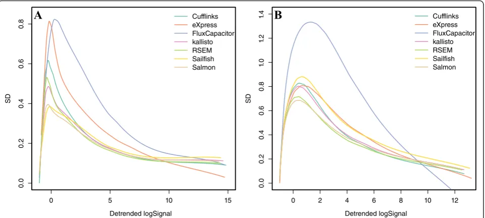
we apply loess [32] to estimate this function. We can then plot several curves on the same plot to compare methods (Fig. 3). To provide summary statistics that take into account the dependence on abundance, we report the median si for low (A lower than 1), medium (A

be-tween 1 and 6), and high (A larger than 6) strata (columns 2–4 in Tables 1 and 2). We include standard error esti-mates of these metrics as well.

In the first dataset, Flux Capacitor and eXpress clearly underperform compared with the other methods in the regions with most data (Abetween 3 and 8). In the sec-ond dataset, only Flux Capacitor clearly underperforms. The other methods performed similarly, with RSEM per-forming slightly better in both datasets. Overall, the pre-cision was substantially worse than what we observe for microarrays (compare, for example, with Fig. 2 in [31]). This is particularly true for low abundance transcripts where even the best methods show a standard deviation of 0.5, which translates to a difference of 41 % between replicate measurements.

Although we observed differences between quantifica-tion algorithms, different aligners show similar results (Additional file 1: Figure S4). STAR generally outper-formed TopHat2, although very marginally. Also, RSEM mapped with Bowtie2 outperformed RSEM with STAR (Additional file 1: Figure S4a).

Because a large percentage of the quantifications are 0, we also developed summary statistics and visualization techniques to assess the across-replicate consistency of 0 calls. Note that the features considered here are those with at least one 0 in the pair of replicated measures. For each of these we report the proportion of discordant calls:

Dið Þ ¼K Pr Ygi1<KYgi2≥K

or Ygi1≥K Ygi2<K

whereKis a threshold defining a transcript as expressed. Because methods that call more 0s are less likely to be discordant, we plot Di(K) against the proportion of the transcript (Fig. 4). The results here are similar to those

of Fig. 3. We report Di(K) for K= 1 in column 5 of

Tables 1 and 2. In both datasets we see Flux Capacitor as clearly underperforming compared with the other methods.

Consistency of isoform calls

Because RNA-seq is commonly used to infer alternative transcription, we also assessed the reproducibility of abundance within transcripts of the same gene. To pro-vide a simple and interpretable metric we considered only the genes with exactly two transcripts. Specifically, for each sample we computed the percentage of reported abundances for each of the first transcripts. So if t1and t2are the reported abundances for transcripts 1 and 2,

we compute t1/(t1+t2). We then performed every

pair-wise comparison of two replicates and for each gene re-corded the difference in these proportions. Note that we expect this difference to be 0 since the same transcripts should be reported in two replicates. We plotted these differences against abundanceAgijsince we expected

lar-ger differences at lower abundances (Additional file 1: Figure S3b). We then stratified the absolute differences by values of Agij and computed the median value. This

permitted us to compare curves across methods (Fig. 5). Here we found Flux Capacitor to underperform com-pared with the other methods, which performed simi-larly. However, it is worth noting how high these values

are, especially for low abundance transcripts where the median differences are close to 0.5, meaning that we are basically guessing which transcript is present.

Sensitivity

The above-described metrics relate to reproducibility or specificity. But given the specificity and sensitivity trade-off, it is imperative that we also assess sensitivity. For ex-ample, a method that calls every gene expressed at 10 TPM has perfect specificity, but would, of course, fail to detect any real differences. Recall that for the first data-set we defined truly differentially expressed genes, not transcripts. For each algorithm, therefore, one measure was constructed for each gene by combining the re-ported quantities for each transcript using the aggrega-tion method recommended by said algorithm. For the second dataset, defining transcripts that were truly dif-ferentially expressed was known by construction.

To assess accuracy, we computed an average log fold change for each of the truly differentially expressed transcripts:

Mg¼1=J2 XJ2

j¼1

log2Yg2jþ0:5

−1=J1 XJ1

j¼1

log2Yg1jþ0:5

;

multiplied it by the sign of the true fold change (so that all true fold changes could be considered positive), and plotted it against the average abundance (Additional file1: Figure S3c):

Fig. 3Standard deviations of transcript quantifications based onaan experimental dataset (GM12878) andba simulation dataset (one of the cell lines). Seven quantification methods are shown here

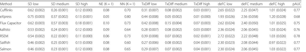
Table 1Summarized metrics for analyzed pipelines based on an experimental dataset

Method SD low SD medium SD high NE (K = 1) NN (K = 1) TxDiff low TxDiff medium TxDiff high deFC low deFC medium deFC high pAUC

Cufflinks 0.62 (0.002) 0.26 (0.001) 0.12 (0.000) 0.08 0.70 0.31 (0.007) 0.08 (0.002) 0.03 (0.001) 2.65 (0.022) 2.25 (0.047) 1.01 (0.024) 0.77

eXpress 0.75 (0.003) 0.37 (0.002) 0.13 (0.001) 0.05 0.80 0.44 (0.008) 0.05 (0.002) 0.01 (0.000) 1.93 (0.026) 2.56 (0.058) 1.20 (0.028) 0.68

Flux Capacitor 0.62 (0.003) 0.57 (0.003) 0.18 (0.001) 0.10 0.73 0.42 (0.008) 0.15 (0.004) 0.07 (0.003) 2.62 (0.024) 2.40 (0.050) 1.01 (0.025) 0.75

kallisto 0.53 (0.002) 0.24 (0.001) 0.12 (0.000) 0.09 0.64 0.28 (0.007) 0.08 (0.002) 0.03 (0.0001 2.36 (0.024) 2.06 (0.045) 1.03 (0.024) 0.76

RSEM 0.54 (0.002) 0.22 (0.001) 0.11 (0.000) 0.06 0.73 0.39 (0.008) 0.07 (0.002) 0.02 (0.001) 2.72 (0.022) 2.22 (0.048) 1.03 (0.026) 0.78

Sailfish 0.46 (0.002) 0.25 (0.001) 0.13 (0.000) 0.08 0.60 0.27 (0.006) 0.08 (0.002) 0.04 (0.001) 2.30 (0.023) 2.08 (0.044) 0.97 (0.022) 0.77

Salmon 0.46 (0.002) 0.23 (0.001) 0.12 (0.000) 0.08 0.65 0.29 (0.007) 0.07 (0.002) 0.04 (0.001) 2.30 (0.024) 2.06 (0.045) 1.03 (0.022) 0.77

Metrics for single cell lines are averaged for both cell lines, except standard deviation is the square root of average squares. Columns 2–4 shows median standard deviation on three transcript abundance levels; column 5 shows proportions of discordant calls when K = 1; column 6 shows proportions of both non-expressed when K = 1; columns 7–9 show the mean proportion differences of transcripts in genes only having two annotated transcripts based on three transcript abundance levels; columns 10–12 show median log fold changes of true differentially expressed genes based on three abundance levels; column 13 shows standardized partial area under the curve for differential expression of genes.pAUCpartial area under the receiver operating characteristic curve

Teng

et

al.

Genome

Biology

(2016) 17:74

Page

6

of

Table 2Summarized metrics for analyzed pipelines based on a simulation dataset

Method SD low SD medium SD high NE (K = 1) NN (K = 1) TxDiff low TxDiff medium TxDiff high deFC low deFC medium deFC high pAUC

Cufflinks 0.73 (0.002) 0.54 (0.003) 0.26 (0.001) 0.090 0.657 0.34 (0.011) 0.08 (0.003) 0.05 (0.003) 0.53 (0.009) 0.95 (0.006) 0.98 (0.003) 0.61

eXpress 0.71 (0.003) 0.67 (0.004) 0.30 (0.001) 0.09 0.68 0.33 (0.009) 0.07 (0.003) 0.07 (0.003) 0.47 (0.011) 0.87 (0.015) 0.91 (0.012) 0.60

Flux Capacitor 1.03 (0.004) 1.23 (0.007) 0.40 (0.002) 0.15 0.63 0.46 (0.013) 0.15 (0.006) 0.07 (0.004) 0.39 (0.011) 0.82 (0.013) 0.97 (0.009) 0.52

Kallisto 0.72 (0.003) 0.55 (0.003) 0.27 (0.001) 0.10 0.63 0.37 (0.011) 0.08 (0.004) 0.05 (0.003) 0.56 (0.008) 0.95 (0.006) 0.98 (0.002) 0.58

RSEM 0.65 (0.002) 0.48 (0.003) 0.25 (0.001) 0.08 0.69 0.43 (0.011) 0.07 (0.004) 0.04 (0.003) 0.58 (0.008) 0.96 (0.006) 1.00 (0.003) 0.65

Sailfish 0.76 (0.003) 0.65 (0.004) 0.30 (0.001) 0.11 0.57 0.34 (0.009) 0.08 (0.004) 0.05 (0.003) 0.52 (0.011) 0.94 (0.011) 0.96 (0.006) 0.56

Salmon 0.64 (0.002) 0.52 (0.003) 0.26 (0.001) 0.09 0.67 0.35 (0.010) 0.08 (0.004) 0.05 (0.003) 0.54 (0.008) 0.95 (0.007) 1.00 (0.003) 0.61

The last four columns are based on differential expression of transcripts.pAUCpartial area under the receiver operating characteristic curve

Teng

et

al.

Genome

Biology

(2016) 17:74

Page

7

of

Ag¼1=2J2 XJ2

j¼1

log₂Yg2jþ0:5

þ1=2J1 XJ1

j¼1

log₂Yg1jþ0:5

To be able to compare methods, we fitted loess curves to these plots and show the curves for all methods. Note that for the second dataset these curves should be equal to 1 for all values of A since all truly differentially expressed transcripts were designed to have true log (base 2) fold changes of 1 (Additional file 1: Figure S5). Here we can see that, with the exception of the

underperformance of Flux Capacitor, all methods perform similarly. As we did for the standard deviation metric, we report the median sensitivity measure for three strata of abundance (columns 10–12 in Tables 1 and 2).

ROC curves and pAUC

Finally, to assess sensitivity and specificity simultan-eously, we constructed receiver operating characteristic (ROC) curves. Because in the first dataset we used genes and in the second we used transcripts, here we use the

Fig. 5Proportion differences of transcript quantifications in genes with only two annotated transcripts based onaan experimental dataset (GM12878) andba simulation dataset (one of the cell lines). Seven quantification methods are shown

Fig. 4Proportions of discordant expression calls based onaan experimental dataset (GM12878) andba simulation dataset (one of the cell lines). Seven quantification methods are shown here

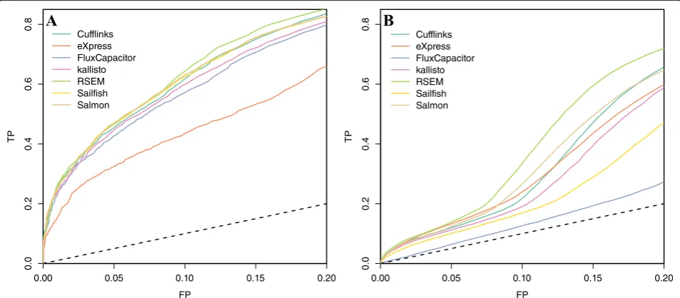
general term featureto refer to both. We used the same approach as in the previous section to define positives (truly differentially expressed features) and negatives (not differentially expressed features). We then obtained log fold change values for every feature across every pairwise comparison between the two groups. Following common practice, we removed all features with both values below 1. Each of these resulted in one ROC curve. We averaged these results using threshold averaging based on fold changes [33] to produce one ROC curve for each method (Fig. 6). The ROC curves only include false positive rates (FPRs) below 0.2 because, in practice, it would be rare to accept a FPR higher than this since a FPR of 0.2 already represents thousands of false positive features. Here we see Flux Capacitor and eXpress under-performing and RSEM slightly outunder-performing the other methods in both datasets. The partial (up to FPR of 0.2) area under the curve (pAUC) is included in column 13 of Tables 1 and 2, which is the standardized area under the curve [34].

Although the results for genes are comparable to those seen for microarrays (see Fig. 4 in [8]), we note that the results for transcripts are not impressive in general. For example, to recover half of the real differences, we need to accept a FPR of over 0.15. In fact, to achieve even these results, we removed all transcripts for which both samples were reporting quantities below 1. Without this filtering, the technology does not perform much better than guessing (Additional file 1: Figure S6). This result is in agreement with a recent publication describing the importance of filtering low abundance values in RNA-seq data [35].

Discussion

Note that for the ROC analysis we show results for both gene level and transcript level analysis and the transcript level metrics were substantially worse (Fig. 6). Previous publications [5] focusing on abundance found that all al-gorithms performed well. Here we found that if your focus is differential expression, then results are not as impressive and differences are found across algorithms.

We do not intend our study of seven methods to be considered a definitive comparison but rather a demon-stration of how one can use simple datasets and inter-pretable metrics to assess algorithms. For this reason, we have created a webtool that permits the comparison of other methods. Furthermore, we make the software used by this webtool freely available so others can compare methods, including new ones. We note here that the webtool includes a third dataset in which batch effects are completely confounded with group. In the future, this dataset will permit the assessment of methods that adjust for batch. An important contribution is that we have fixed assessments, making it harder for developers to fall into the self-assessment trap.

Finally, note that our method is meant to assess the quantification method specifically. Because, in general, our method does not consider biological replicates, it is not meant to be used for comparisons of statistical methods such as DESeq2 [36] and edgeR [37].

Conclusions

We have described a series of metrics and visualization techniques that facilitate the statistical evaluation of al-gorithms for processing RNA-seq data. The method is

Fig. 6ROC curves indicating performance of quantification methods based on differential expression analysis ofaan experimental dataset and ba simulation dataset. Seven quantification methods are shown.FPfalse positive,TPtrue positive

applicable with a small experiment involving as few as two sets of replicates and data from an independent platform. Using this approach, we assessed several com-peting approaches in terms of specificity and sensitivity. With the exception of the underperforming Flux Capacitor and eXpress, we found that the other algorithms performed similarly. We found that overall performance in detecting differentially expressed transcripts was poor. We also found that the mapping algorithms had a comparatively small effect, with STAR slightly outperforming TopHat2 when compared directly.

Methods Cell line data

The dataset used in this comparison was derived from two widely studied cell lines: GM12878 and K562. The RNA-seq data are described by the ENCODE data center (https://www.encodeproject.org/) with dataset accession IDs ENCSR000AED and ENCSR000AEM. Microarray data for these two cell lines were downloaded from GEO with accession ID GSE26312 [38].

Quasi-simulated dataset

The GENCODE v16 GTF file was downloaded from GENCODE (http://www.gencodegenes.org/) and all protein-coding genes from chromosome 2 with a single isoform or two isoforms were extracted; in addition, 300 genes with 3–15 isoforms were sampled. These genes were used to create a set of transcripts (all the isoforms from the selected genes) from which paired-end reads would be simulated. FPKM values for genes were sam-pled from the empirical distribution of FPKM values for genes estimated by Cufflinks [13] on the 30 Geuvadis samples, excluding values of FPKM less than 1.8. Ex-pression was distributed randomly to the isoforms within a gene using a flat Dirichlet distribution.

The simulated reads were generated using the Polyes-ter software [25], with a modification to allow for fragment-level GC content bias described below. Paired-end reads were generated assuming an experiment with 30 million reads in total, then scaled down for the simu-lated samples, which corresponded to Geuvadis samples with lower sequencing depth, and scaled up for the sim-ulated samples corresponding to Geuvadis samples with higher sequencing depth. The scaling was chosen based on the total number of pairs which both aligned using TopHat2 [11]. The fragment length distribution for the simulated paired-end reads was centered at 160 bp and with a SD of 30 bp, chosen to match the fragment width distribution in the 30 Geuvadis samples.

The samples were distributed using a block design with 15 samples in a simulated condition 1 (seven from batch 1 and eight from batch 2) and 15 samples in a simulated con-dition 2 (eight from batch 1 and seven from batch 2). The

bias parameters used to simulate fragment GC bias were drawn directly from the values estimated on the corre-sponding Geuvadis sample using the alpine software [39]. For 80 % of genes, one of the conditions had the expected mean value multiplied by 2, for 10 % of genes one of the conditions had the expected value equal to 0, and the remaining 10 % of genes represented the null, having no difference in expected value for the mean across conditions. Fragments generated by Polyester were randomly dis-carded using Bernoulli trials, with the probability of suc-cess given by the estimated dependence of the fragment rate on GC content, as estimated by alpine [39]. As this resulted in less fragments than the original target, the simulation was repeated again, scaling proportionally such that the original target sequencing depth would be reached.

Transcript annotation

Although the methodology described here can be gener-ally applied to any set of features, for the comparison carried out here we quantified expression levels for tran-scripts annotated in the GENCODE v16 database [40]. Note that this database includes protein-coding genes, pseudogenes, long non-coding genes (lncRNAs), and others. We focused on protein-coding genes to illustrate our proposed metrics. The units used by the quantifica-tion profiles of protein coding genes can be in reads per kilobase of exon per million reads mapped (RPKM), fragments per kilobase of exon per million fragments mapped (FPKM) or transcripts per million (TPM), etc., depending on the pipelines.

Data quantification and preprocessing

All the RNA-seq samples were first aligned with STAR (version 2.3.1) and Bowtie2 (version 2.2.1). The dataset containing GM12878 and K562 was aligned with TopHat2 (version 2.0.8) as well. Quantification pipelines, including Cufflinks (version 2.2.1), eXpress (version 1.5.1), Flux Capacitor (version 1.5.1), kallisto (version 0.42.3), RSEM (version 1.2.11), Sailfish (version 0.6.2), and Salmon (version 0.5.0) were used to quantify transcript expression levels, represented by units of FPKM, RPKM, or TPM. For more details, such as the commands and parameter set-tings, refer to the log information on the webtool. RMA [41] was used to normalize microarray samples between two cell lines and corresponding replicates.

Correlation is not a measure of reproducibility

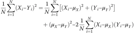
For lists of numbers to be considered to reproduce an-other, the differences between the entries of the list must be close to 0. We can summarize with one number by using distance. Note that distance and correlation are re-lated. We can rewrite the distance (squared and divided byN) between two vectorsXandY:

1 N

XN

i¼1

Xi−Yi

ð Þ2

as:

1 N

XN

i¼1

Xi−μX

ð Þ−ðYi−μYÞ þðμX−μYÞ

½ 2

where μXis the average of theXs andμYis the average of theYs. Then we have:

1 N

XN

i¼1

Xi−Yi

ð Þ2_¼ 1

N XN

i¼1

Xi−μX

ð Þ2_þ

Yi−μY

ð Þ2

þðμX−μYÞ

2₋

21 N

XN

i¼1

Xi−μX

ð ÞðYi−μYÞ

Note that the last term is the covariance. To simplify this equation assume that X and Y have been standard-ized to have standard deviation 1. Then the equation re-duces to:

1 N

XN

i¼1

ðXi−YiÞ2¼2þ ðμX−μYÞ

2₋

2⋅correlation

and we see the direct relationship between distance and correlation. However, an important difference is that the distance contains the term (μX−μY)2and can therefore detect cases that are not reproducible due to large aver-age changes. These could happen, for example, if the data are not properly normalized.

The above calculation can be re-expressed in a way that shows yet another flaw with correlation as a meas-ure of reproducibility. Suppose you have a series of mea-surements X and a second measurement differs by d. We want the variability of d to be as small as possible. However, the correlation betweenXandX+dcan be re-written as:

corrðX;XþdÞ ¼ ffiffiffiffiffiffiffiffiffiffiffiffiffiffiffiffiffiffiffiffiffiffiffiffiffiffiffiffiffiffiffiffiffiffiffiffiffi1 1þvarð Þd =varð ÞX p

which implies that if the variability across values of Xis very large, as it is in RNA-seq data, you can have corre-lations close to 1 regardless of the variability of the dif-ference. Note that var(X) is about 4 in a typical RNA-seq experiment. This implies that a var(d) of 1 results in a correlation of almost 0.9. While 0.9 is considered high by biologists, a variance of 1 is not acceptable as it im-plies typical across-replicate fold changes of 2.

Software license

The R/Bioconductor package rnaseqcomp is available under open source license GPL-3.

Additional file

Additional file 1: Figure S1.aA pair of independent normally distributed datasets are simulated. The correlation is 0 by design. The values of one pair were_“accidentally_”changed to be very large, changing the correlation from 0 to 0.9.bFor the data in Figure S2, we computed SD, Pearson correlation, and Spearman correlation metrics. A useful metric will detect the first pair (denoted with atriangle) as different. Note that the SD metric is by far the best at making this distinction. The Pearson correlation for this pair is above 0.9.Figure S2.MA plots for eight pairs of replicates. The first one seems to be problematic as the first replicate is generally larger than the second. The title of each panel shows the SD and demonstrates that this metric does detect the first pair of replicates as being different. Figure S3.Three types of proposed metrics change with transcript abundances. Cufflinks quantifications on a simulation dataset are shown here as an example.aStandard deviation.bProportion differences of transcripts in genes with only two annotated transcripts.cEstimated log fold changes for simulated differentially expressed transcripts.Figure S4. Effects of aligners on four major types of metrics. Quantifications for an experimental dataset from cell lines GM12878 and K562 are shown here as an example. Comparison between STAR and TopHat2 are based on Cufflinks and Flux Capacitor. Comparison between Bowtie2 and STAR are based on RSEM.aStandard deviations based on the cell line GM12878. bProportion of discordant calls.cProportion differences of transcripts in genes with only two annotated transcripts based on cell line GM12878. dROC curves based on transcript fold changes between GM12878 and K562.Figure S5.Log fold changes of true differential expression fitted by loess.aPlot based on experimental dataset from cell lines GM12878 and K562. True differentially expressed genes are estimated using microarray data.bPlot based on simulation dataset with true differentially expressed transcripts predefined.Figure S6.ROC curves on a simulation dataset when no filtering is applied on expression calls. (PDF 1052 kb)

Competing interests

The authors declare that they have no competing interests.

Authors’contributions

MT and RAI developed the benchmarks, wrote the bioconductor package

rnaseqcomp, created the webtool for quantification submission and comparison, and wrote the manuscript. MIL prepared the second simulation dataset. MT, AD, SL, CEM, XW, and RAI made the comparative analysis for initial quantification pipelines. BRG, SO, CAS, and LZ generated data. CAD, SD, and DP provided valuable suggestions for the benchmark and manuscript. All authors read and approved the final manuscript.

Acknowledgements

We thank the ENCODE RNA working group for providing Cufflinks, eXpress, Flux Capacitor, RSEM, and Sailfish quantifications and suggestions regarding metric development. We also thank Dr. Zhiping Weng and Dr. Roderic Guigó for comments on the manuscript.

Author details 1

Department of Biostatistics and Computational Biology, Dana-Farber Cancer Institute, 450 Brookline Avenue, Boston, MA 02215, USA.2_{Department of} Biostatistics, Harvard TH Chan School of Public Health, 677 Huntington Avenue, Boston, MA 02115, USA.3_{Functional Genomics Group, Cold Spring} Harbor Laboratory, 1 Bungtown Road, Cold Spring Harbor, NY 11724, USA. 4_{Bioinformatics and Genomics Programme, Centre for Genomic Regulation} (CRG) and UPF, Doctor Aiguader, 88, Barcelona 08003, Spain.5_{Department of} Genetics and Genome Sciences, Institute for System Genomics, UConn Health Center, Farmington, CT 06030, USA.6Department of Physiology and Biophysics, Weill Cornell Medical College, New York, New York, USA. 7_{Department of Genetics, Stanford University, 300 Pasteur Drive, MC-5477,} Stanford, CA 94305, USA.8_{School of Computer Science and Technology,} Harbin Institute of Technology, Harbin, China.

Received: 6 August 2015 Accepted: 8 April 2016

References

1. Consortium EP. The ENCODE (ENCyclopedia Of DNA Elements) Project. Science. 2004;306:636_–40.

2. Bray N, Pimentel H, Melsted P, Pachter L. Near-optimal probabilistic RNA-Seq quantification. Nat Biotechnol. 2016. doi:10.1038/nbt.3519. 3. Patro R, Mount SM, Kingsford C. Sailfish enables alignment-free isoform

quantification from RNA-seq reads using lightweight algorithms. Nat Biotechnol. 2014;32:462–4.

4. Norel R, Rice JJ, Stolovitzky G. The self-assessment trap: can we all be better than average? Mol Syst Biol. 2011;7:537.

5. Kanitz A, Gypas F, Gruber AJ, Gruber AR, Martin G, Zavolan M. Comparative assessment of methods for the computational inference of transcript isoform abundance from RNA-seq data. Genome Biol. 2015;16:150. 6. Leek JT, Scharpf RB, Bravo HC, Simcha D, Langmead B, Johnson WE, et al.

Tackling the widespread and critical impact of batch effects in high-throughput data. Nat Rev Genet. 2010;11:733_–9.

7. Irizarry RA, Warren D, Spencer F, Kim IF, Biswal S, Frank BC, et al. Multiple-laboratory comparison of microarray platforms. Nat Methods. 2005;2:345–50. 8. Irizarry RA, Wu Z, Jaffee HA. Comparison of Affymetrix GeneChip expression

measures. Bioinformatics. 2006;22:789–94.

9. McCall MN, Irizarry RA. Consolidated strategy for the analysis of microarray spike-in data. Nucleic Acids Res. 2008;36:e108.

10. Dobin A, Davis CA, Schlesinger F, Drenkow J, Zaleski C, Jha S, et al. STAR: ultrafast universal RNA-seq aligner. Bioinformatics. 2013;29:15–21. 11. Kim D, Pertea G, Trapnell C, Pimentel H, Kelley R, Salzberg SL. TopHat2:

accurate alignment of transcriptomes in the presence of insertions, deletions and gene fusions. Genome Biol. 2013;14:R36.

12. Langmead B, Salzberg SL. Fast gapped-read alignment with Bowtie 2. Nat Methods. 2012;9:357_–9.

13. Trapnell C, Williams BA, Pertea G, Mortazavi A, Kwan G, van Baren MJ, et al. Transcript assembly and quantification by RNA-Seq reveals unannotated transcripts and isoform switching during cell differentiation. Nat Biotechnol. 2010;28:511–5.

14. Roberts A, Pachter L. Streaming fragment assignment for real-time analysis of sequencing experiments. Nat Methods. 2013;10:71_–3.

15. Montgomery SB, Sammeth M, Gutierrez-Arcelus M, Lach RP, Ingle C, Nisbett J, et al. Transcriptome genetics using second generation sequencing in a Caucasian population. Nature. 2010;464:773_–7.

16. Li B, Dewey CN. RSEM: accurate transcript quantification from RNA-Seq data with or without a reference genome. BMC Bioinformatics. 2011;12:323. 17. Patro R, Duggal G, Kingsford C. Salmon: accurate, versatile and ultrafast

quantification from RNAseq data using lightweight-alignment. bioRxiv. 2015. doi:10.1101/021592.

18. Mortazavi A, Williams BA, McCue K, Schaeffer L, Wold B. Mapping and quantifying mammalian transcriptomes by RNA-Seq. Nat Methods. 2008;5:621–8.

19. Jiang L, Schlesinger F, Davis CA, Zhang Y, Li R, Salit M, et al. Synthetic spike-in standards for RNA-seq experiments. Genome Res. 2011;21:1543–51. 20. Loven J, Orlando DA, Sigova AA, Lin CY, Rahl PB, Burge CB, et al. Revisiting

global gene expression analysis. Cell. 2012;151:476_–82.

21. Risso D, Ngai J, Speed TP, Dudoit S. Normalization of RNA-seq data using factor analysis of control genes or samples. Nat Biotechnol. 2014;32:896–902. 22. Ritchie ME, Phipson B, Wu D, Hu Y, Law CW, Shi W, et al. limma powers

differential expression analyses for RNA-sequencing and microarray studies. Nucleic Acids Res. 2015;43:e47.

23. Benjamini Y, Hochberg Y. Controlling the false discovery rate: a practical and powerful approach to multiple testing. J R Stat Soc Ser B (Methodological). 1995;57:289–300.

24. Lappalainen T, Sammeth M, Friedlander MR, t Hoen PA, Monlong J, Rivas MA, et al. Transcriptome and genome sequencing uncovers functional variation in humans. Nature. 2013;501:506–11.

25. Frazee AC, Jaffe AE, Langmead B, Leek JT. Polyester: simulating RNA-seq datasets with differential transcript expression. Bioinformatics. 2015;31:2778–84.

26. Eisenberg E, Levanon EY. Human housekeeping genes, revisited. Trends Genet. 2013;29:569_–74.

27. Kumamaru H, Ohkawa Y, Saiwai H, Yamada H, Kubota K, Kobayakawa K, et al. Direct isolation and RNA-seq reveal environment-dependent properties of engrafted neural stem/progenitor cells. Nat Commun.

2012;3:1140.

28. Marinov GK, Williams BA, McCue K, Schroth GP, Gertz J, Myers RM, et al. From single-cell to cell-pool transcriptomes: stochasticity in gene expression and RNA splicing. Genome Res. 2014;24:496–510.

29. Freedman D, Pisani R, Purves R. Statistics. 4th ed. New York: W.W. Norton & Co; 2007.

30. Law CW, Chen Y, Shi W, Smyth GK. voom: Precision weights unlock linear model analysis tools for RNA-seq read counts. Genome Biol. 2014;15:R29. 31. Cope LM, Irizarry RA, Jaffee HA, Wu Z, Speed TP. A benchmark for

Affymetrix GeneChip expression measures. Bioinformatics. 2004;20:323–31. 32. Cleveland WS, Devlin SJ. Locally Weighted Regression: An approach to

regression analysis by local fitting. J Am Stat Assoc. 1988;83:596–610. 33. Fawcett T. An introduction to ROC analysis. Pattern Recogn Lett.

2006;27:861–74.

34. McClish DK. Analyzing a portion of the ROC curve. Med Decis Making. 1989;9:190–5.

35. Soneson C, Matthes KL, Nowicka M, Law CW, Robinson MD. Isoform prefiltering improves performance of count-based methods for analysis of differential transcript usage. Genome Biology. 2016. 17:12. doi: 10.1186/ s13059-015-0862-3.

36. Love MI, Huber W, Anders S. Moderated estimation of fold change and dispersion for RNA-seq data with DESeq2. Genome Biol. 2014;15:550. 37. Robinson MD, McCarthy DJ, Smyth GK. edgeR: a Bioconductor package for

differential expression analysis of digital gene expression data. Bioinformatics. 2010;26:139–40.

38. Ernst J, Kheradpour P, Mikkelsen TS, Shoresh N, Ward LD, Epstein CB, et al. Mapping and analysis of chromatin state dynamics in nine human cell types. Nature. 2011;473:43–9.

39. Love MI, Hogenesch JB, Irizarry RA. Modeling of RNA-seq fragment sequence bias reduces systematic errors in transcript abundance estimation. bioRxiv. 2015. doi: 10.1101/025767.

40. Harrow J, Frankish A, Gonzalez JM, Tapanari E, Diekhans M, Kokocinski F, et al. GENCODE: the reference human genome annotation for The ENCODE Project. Genome Res. 2012;22:1760–74.

41. Irizarry RA, Hobbs B, Collin F, Beazer-Barclay YD, Antonellis KJ, Scherf U, et al. Exploration, normalization, and summaries of high density oligonucleotide array probe level data. Biostatistics. 2003;4:249–64.

• We accept pre-submission inquiries

• Our selector tool helps you to find the most relevant journal • We provide round the clock customer support

• Convenient online submission • Thorough peer review

• Inclusion in PubMed and all major indexing services • Maximum visibility for your research

Submit your manuscript at www.biomedcentral.com/submit

Submit your next manuscript to BioMed Central

and we will help you at every step: