Development of Analogue Computer for the Simulation of Linear Circuits and Systems

(1)

(2)

Technology (IJRASET)

©IJRASET 2015: All Rights are Reserved

97

Development of Analogue Computer for the

Simulation of Linear Circuits and Systems

Rufus Sola Fayose

Department of Physics and Electronics, Adekunle Ajasin University, Akungba Akoko, Nigeria

Abstract-In order to better understand the physical world, scientists use mathematical models to predict the reaction of various physical systems, such as the motion of a mass attached to a spring, to external stimuli. Such systems are reduced appropriate differential equations. However, to actually show graphical representation of the solutions to these models becomes computationally complex. An analogue computer consisting summers, integrators and coefficient potentiometer was constructed to solve this problem. Using different types of differential equations and assuming different initial conditions the system’s response to sine, triangle and square waves of frequencies between 2Hz to 10KHz were determined. Applying the computer to a control transfer function, the response was obtained for different values of gain K from 0.3 to 0.9, it was shown that the overshoot, the delay time, the rise time, settling time and frequency response all vary significantly with K. The analogue computer system designed includes the following major units: summers, integrators and coefficient potentiometers. Also, sine wave, square wave, and triangular wave at low frequency from 0.01Hz to 200Hz were included in the design. A computer switch mode power supply was used as the dc voltage source. The output from the analogue computer is in the form of a voltage, which must be read and recorded by the use of oscilloscope or X-Y plotter.

Keywords: Analogue Computer, Transfer Function, Control System

I. INTRODUCTION

The analogue computer is a device, which simulates the variables of a system in terms of similar physical quantities easy to generate and control continuously. The analogue computer is basically an electronic simulator in which continuously varying voltages are used to represent the system variable such as temperature, pressure, velocity etc the independent variable being the time (Korn et. al., 1956). In solving such a problem physical quantities are translated into related mechanical or electrical quantities and uses mechanical or electrical equivalent circuits as an analogue for the physical phenomenon being investigated. Analogue computer is a computer that operates on analogue data by performing physical process on the data. An analogue computer comprises of a patch board that provides connections to large numbers of integrators, amplifiers and potentiometers (Howe, 1961). Adjusting the values of the potentiometers enables the gain of the amplifiers and the time constants of the integrators to be varied. Each amplifier or integrator has a summing junction, thus allowing several input signals to be connected to these devices. The variables of a control system are represented on an analogue computer by the output voltages of the amplifiers and integrators (Nelson, 1996):

Analogue computers are very useful for solving mathematical equations, which describe the behaviour of a system. It is used extensively in the study of system dynamics; that is, the study of the transient and steady-state behavior of a wide variety of physical systems (Horowitz and Hill, 1995). Today all analogue computers are electronic and the quantity used is voltage. For example consider the differential equation:

This equation is merely a mathematical expression and is not necessarily related to electrical quantities. Suppose it is assumed that y

is a voltage, then

dt

dy

, 2 2

dt

y

d

,

cSin



t

would also be voltages.

Though differential equations contain derivatives, mathematical differentiations are almost never performed on an analogue computer because differentiation produces voltages whose amplitudes are proportional to their frequencies. It in effect, amplifies high frequency noise to an unacceptable level. The basic mathematical operations like Summation, Integration, and multiplication

1

2 2

t

cSin

by

dt

dy

a

dt

y

d



(3)

Technology (IJRASET)

98

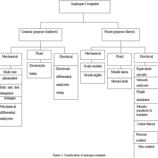
[image:3.612.30.582.95.646.2]

are performed on an analogue computer (McKenzie, 1967)

Figure 1: Classification of analogue computer

The scope of this research work is to design and construct an analogue computer to solve the following type of differential equations.

)

(

)

(

₂ ₂ ₃

2 1 2 2

t

f

x

a

dt

dx

a

dt

y

d

a

dt

x

d

i





Analogue Computer

General purpose (indirect)

Fixed purpose (direct)

Mechanical

Fluid

Electrical

Mechanical

Fluid

Electrical

Slide rule

planimeter

(4)

Technology (IJRASET)

99

II. DIFFERENTIAL EQUATION

A differential equation is an equation that describes the relationship between an unknown function and its derivatives. It describes the relationship between an independent varable,x, a dependent variable y, and one or more derivatives of y with respect to x (Rummer, 1969)

Differential equations represent dynamic relationships, such as, quantities that change, and frequently occur in scientific and engineering problems. The order of a differential equation is the highest order derivative involved in the equation (Stroud, 2005.

An important special case is when the equation does not involve x. This differential equation may be represented as a vector field. This type of differential equations has the property that space can be divided into equivalent classes based on whether two points lie on the same solution curve. Since the laws of physics are believed not to change with time, the physical world is governed by such differential equations (McDonald and Howe 2000). The problem of solving a differential equation is to find the function y whose derivatives satisfy the equation.

III. METHODOLOGY

An equation was solved on an analogue computer by using operations (such as addition, subtraction, integrations) on voltages that represent the variables of the equation. The amplifiers are connected together in such a way that the mathematical relations prescribed by the equation are performed and a time-varying voltage is measured to obtain the solution. In the design each integrator is a four input summing-integrator circuit. Polycarbonate capacitor (PCC) was used as feedback component because it has a tolerance value of



1 %

which is very good for signal processing. Selecting 1f polycarbonate capacitor, the resistor value can be calculated thus.

Using,

where K is the gain of the integrator,

when K = 1

Also when K = 2,

similarly, when K = 5, R = 200kΩ and when K = 10, R = 100kΩ.

IV. SOLVING PROBLEMS WITH THE ANALOGUE COMPUTER

The analogue computer designed was used to solve a wide variety of problems including nonlinear functions and time-dependent coefficients. The equations solved are linear, constant-coefficient, differential equations, which describe the behaviour of linear,

0 )

(

2 5 6 7

2 4 2 2





a

y

dt

dx

a

dt

dy

a

dt

x

d

a

dt

y

d

ii

)

2 .

0

1 )(

1 (

)

(

s

K

G

iii





3

0

2 2





e

x

dx

dy

y

dx

y

d

xy

0 sin

2





y

x

dx

dy

x

2 



_

M

(5)

Technology (IJRASET)

100

time-invariant, control system (Weyrick, 1969).

Usually the problems to be solved measure or record the response of a control system to the application of a particular input signal. The problem was solved by modeling the control system on the analogue computer, applying relevant input signals and recording the voltage output representing the control system response (Peterson, 1967).

Amplifiers, integrators and potentiometers were used to construct the model and the system differential equation dictates the way in which these components are connected together to simulate the control system (Odo, 2002).

V. THE X-Y PLOTTER

The X-Y plotter used was an electromechanical device, which gives good recordings of two variables against each other. It consisted of two position mechanisms controlling the motion of a pen over a chart. The two axes of motion are perpendicular to each other and correspond to the X and Y coordinates. A simple X-Y plotter consisted of a pen, which was driven, in the Y direction by one servo-motor mounted on the pen carriage. A second servo-motor controls the displacement of the pen carriage in the X direction. The X and Y inputs have different frequency responses because of large difference in the mass of the two servo systems. Time-base units were normally incorporated in X-Y plotters to give Y-t or X-t plots where desired. It produced X-Y plots of one variable against another variable. However the major disadvantage was the relatively poor speed of response, due to the inertia of the moving parts.

VI. SIMULATION

Before wiring the analogue computer to solve differential equations, certain procedures leading to a wiring diagram were followed. The process is outlined is as follows:

The differential equation is manipulated to solve for the highest order derivative present in the equation. It is assumed that a voltage representing the highest order derivative is available.

With the assumption of step 2, the equation is integrated to produce a voltage representing the next lower order derivative. The integrator is drawn and labeled showing its output with the next lower order derivative (including a minus sign for the phase inversion caused by the integrator)

Additional integrators and amplifiers are drawn which are necessary to generate all variables in the differential equation. These are combined in accordance with the equation obtained in step 1.

When all the voltages representing all the terms on the right side of the equation in step 1 have been summed together, the result is equal to the highest order derivative that we assumed we had in step 2. Therefore, this sum of terms is connected to the input of the first integrator (the one in step 3).

Following the above procedure, the analogue computer constructed was used to solve the Simultaneous Differential equations and Control Transfer function

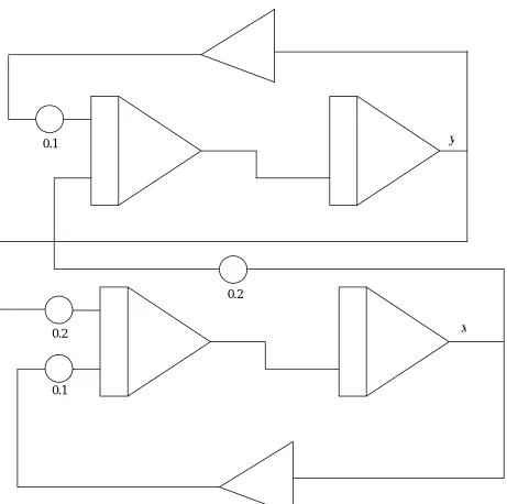
Consider the Simultaneous Differential equations

This simultaneous differential equation was solved using the constructed analogue computer. The flow diagram for the simultaneous differential equation is shown in figure 2

The signal output obtained from an X-Y plotter of the flow diagram of figure 2 is shown in figure 3. The result obtained as shown on the X-Y plotter was in agreement with the expected waveform.

0

2

0

2

2 2













x

y

dt

y

d

y

x

dt

x

d

(6)

Technology (IJRASET)

[image:6.612.59.520.77.535.2]

101

Figure 2: Analogue Computer flow diagram for solving the equation 8

Figure 3: Response obtained from X-Y plotter for the simultaneous differential equation 4 and 5

1 . 0

2 .

0 x

y

2 . 0

[image:6.612.182.414.562.705.2]

(7)

Technology (IJRASET)

102

Similarly considered the Control Transfer function

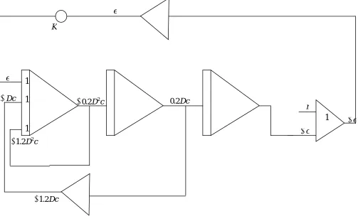
The transfer function was turned into differential equation yielding

Solving this

equation for the highest-order derivatives gives

The flow diagram for equations 8 is shown in figure 4.

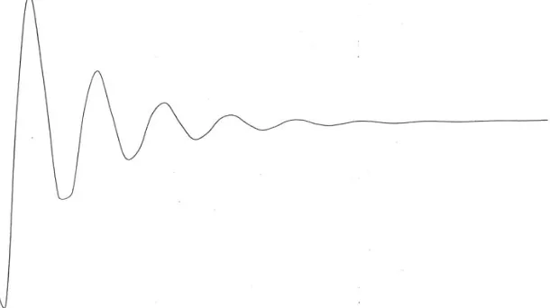
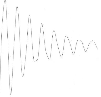
[image:7.612.60.563.309.620.2]

Figures 5 to 9 shows the signal outputs obtained from an X-Y plotter at different values of the gain (K) ranging from 0.3 to 0.9. The overshoot, delay time, rise time, settling time and frequency response for the various values of the gain K are given in Table 1

Figure 4: Analogue Computer setup of equations 6 and 7

The accuracy of an analogue computer simulation was found to depend on the quality of the computing amplifiers, the tolerance of components, the potentiometers settings, the accuracy of the output devices and the problem itself.

)

2 .

0

1 (

)

1 (

s

K

G





7 e

c

r





6

2 .

1

2 .

0 D

3

c



D

2

c



Dc



Ke

8

2 .

1

2 .

0

3 2

Dc

c

D

Ke

c

D





r e  c D2 2 . 0

(8)

Technology (IJRASET)

[image:8.612.174.424.85.251.2]

103

Figure 5: Response of the Control Transfer Function of equation 8 with gain of 0.3 as displayed by X-Y plotter

[image:8.612.169.474.288.459.2]

(9)

Technology (IJRASET)

[image:9.612.119.455.92.227.2]

104

[image:9.612.167.478.260.438.2]

[image:9.612.183.395.471.676.2]

(10)

Technology (IJRASET)

105

Table: 1: Response of control Transfer Function at different values of gain K K=0.3 K= 0.5 K = 0.6 K = 0.7 K = 0.9

Overshoot 0.25% 5.00% 6.25% 6.435% 9.75% Delay Time 0.10s 0.15s 0.20s 0.10s 0.00s Rise Time 0.18s 0.10s 0.15s 0.12s 0.00s Settling Time 0.30s 2.30s 5.95s 0.00s 0.00s Freq. Response 1.18Hz 1.11Hz 0.59Hz 1.60Hz 1.54Hz

VII. RESULTS AND DISCUSSION

From the response of the different signals (Square wave, Sine wave and Triangular wave) applied as the forcing functions, the output tried to match the input waveform for every wave that we put into the system. This is most noticeable at low frequency around 20Hz. It was noticed that the output can never really match the input. When triangular waves and sine waves are put into the circuit, the inability to match the input results in a phase shift. In every case, as the frequency increased, the phase change also increased. The X-Y plotter used to produce the graphs could not sample fast enough, but the reaction at low frequency for all waves was really interesting. This phase shift, and inability to match the input can be described in a couple of different ways. In physics terms, this shift is the momentum of the mass that is attached to the spring. As the input wave changes values, the mass cannot instantaneously follow. Because of its momentum, it must first be brought to rest and then start moving in the other direction. In systems terms, the phase shift is simply a result of the circuit. The circuit does not have a completely linear phase, and this non-linear phase will cause distortions in any waveform as it travels through the circuit.

The response obtained from X-Y plotter for the simultaneous differential equation 4 and 5 shown in figure 3 shows that the nature of the waveform looks like sine wave. From the figure 3 wave x is leading y by 1030, which was in complete agreement to the solution of equations 4 and 5.

The response of the Control Transfer Function of equation 8 as displayed on an X-Y plotter is shown in figure 5 to 9.The desired value of the gain is selected by adjusting the setting of the potentiometer. Varying the values of the gain K the overshoot, delay time, rise time, settling time and the frequency response of each of the waveform is obtained which is shown in table 3.1. When the gain K = 0.3 the overshoot, delay time, rise time, settling time and frequency response was 0.25%, 0.10s, 0.18s, 0.30s and 1.18Hz. Also when the gain K = 0.5 the overshoot, delay time, rise time, settling time and frequency response was 5.00%, 0.15s, 0.10s, 2.30s and 1.11Hz respectively. Similarly when gain K = 0.6 the overshoot, delay time, rise time, settling time and frequency response were respectively 6.25%, 0.20s, 0.15s, 5.95s and 0.59Hz. The result obtained shows that the peak overshoot varies directly as the gain, that is, the peak overshoot increases as the gain increases. Analogue simulation of a control system is a useful way to investigate the stability, peak overshoot and the settling time of the system. The output of a stable control system ultimately reaches and maintains some steady-state position while the output of an unstable system oscillates indefinitely.

VIII. CONCLUSION AND RECOMMENDATION

After adjusting our design, it was found that the analogue computer efficiently gave solutions to the differential equation that we were trying to solve. Analogue computers are definitely not as accurate as digital computers, but they are incredibly fast at solving differential equations. Because analogue computers solve differential equations speedily, the frequency or shape of the forcing function could be changed; the output waveform is produced with an unnoticeable delay.

Another advantage of analogue computer simulation is that solution to problems are produced in real time which implies that solutions can be time-scaled so that they occur in either “fast time” or “slow time”

(11)

Technology (IJRASET)

106

at different points in the circuit.

However, there are disadvantages to analogue computers. The principal disadvantage is that the user must be reasonably well acquainted with the computer hardware for a maximally effective simulation. He must be aware of amplifier limitations, noise sources, frequency response and the capabilities and operations of the output display devices.

In the end, analogue computers are an effective way to model real world physical systems. Analogue computers are also very useful in simulation in that the results are usually presented in the form of a continuous graph of the required variables and the system performance is easily observable. It is useful in the real time solution of differential equation.

REFERENCES

[1] D’azzo J.J. and Houpis C.H. (1960): Feedback control System Analysis and Synthesis. McGraw-Hill Book Company. Inc. pp 72-86 [2] Franco S. (1998): Designing with Operational Amplifier and Analog Integrated Circuits McGraw-Hill Company USA pp 4-35 [3] Henry J and Leslie B. (1974): Electronic Computers made simple. W.H Allen & company, Ltd, London pp 83

[4] Herrick C.N. (1974): Electronic Service Instruments. Prentice-hall, Inc. pp 32-51

[5] Horowitz P and Hill, W. (1995): The art of Electronics. Second edition. Cambriage University Press, Cambridge, UK. Pp 90 [6] Howe, R.M. (1961): Design Fundamentals of Analog computer Components. New Jersey:

[7] D. Van Nostrand Company. Inc. pp 62

[8] John, V.W., Lawrence P.H and Granino, A.K. (1992): Introduction to operational Amplifier Theory and Application. McGraw-Hill book Company, Inc. pp 43 [9] Korn, Granino A. korn, Theresa M. (1956): Electronic Analog Computers: (D-C Analog Computers). 2nd_{Ed. New York: McGraw-Hill Book Company, Inc. 21}

- 69

[10] McDonald A.C. and Howe H (2000): Feedback and control Systems pp 54

[11] McKenzie, A. (1967): Analog Computer Applications. A Symposium Held at Paisley College of Technology. London: Sir Isaac Pitman and Sons Ltd. Pp 4 - 7 [12] Millman J. and Halkians C.C. (1972): Integrated Electronics: Analog and Digital Circuits and Syatems. Mcgraw-Hill Company. pp 88

[13] Nelson J.C.C. (1996): Basic Operational Amplifiers. Butterworth & Co Ltd. Pp 9

[14] Odo, E.A. (2002): Precision thermometric system using Radio telemetry with Computer Interfacing M Tech Thesis submitted to Federal University of Technology, Akure. Pp 10 - 31

[15] Oroge, C.O. (1986): Control System Engineering. University Press limited Ibadan. Pp 22

[16] Pericles E. and Edward Leff. (1979): Introduction to Feedback control Systems. McGraw-Hill Book company, Inc. pp 40 [17] Peterson, Gerald R (1967): Basic Analog computation. The Macmillan Company New York. Pp 32

[18] Rummer, Dele I. (1969) Introduction to Analog computer Programming. Dallas: Holt Rinehart and Winston, Inc. pp 6 [19] Stroud K.A. (1996): Further engineering Mathematics Palgrave publishing New York. Pp 78

[20] Weyrick, Robert C. (1969) Fundamentals of Analog Computers. New Jersey: Prentice-Hall, Inc. pp 9 [21] Wheeler G.J. (1972): Electronic assembly and Fabrication. Reston publication Co. Reston. Pp 55 [22] Wheeler G.J. (1972): The design of Electronic Equipments Prentice-hall, Inc. pp 6

(12)