Technology (IJRASET)
Design of Robust Pi/Pid Controller for Two input
Two Output Gas Turbine Application
Ch.Badri Vishal1, Dr. M Siva Kumar 2 T.Bala Bhargavi 3, 1
PG student, EEE Department, Gudlavalleru Engineering College (JNTUK), Gudlavalleru, AP, India.
2
Professor & HOD, EEE Department, Gudlavalleru Engineering College, Gudlavalleru, AP, India.
3
Assistant professor, EEE Department, Gudlavalleru Engineering College, Gudlavalleru, AP, India.
Abstract: - In this paper, design of pi/pid controllers for the gas turbine application is proposed. The gas turbine application considered here is a TITO system which has two inputs and two outputs. In most of the industrial applications controllers are of pid type. In this paper a new interval analysis method is proposed for the design of robust pi/pid controllers. This method uses the robust stability conditions to derive necessary and sufficient conditions for the stability of interval systems. These conditions are used to get the inequality constraints in terms of controller parameters. The constraints derived are solved using MATLAB. The optimum controller parameters are obtained using this method. The simulation results of the gas turbine application successfully verified and show the efficacy of the proposed method.
Keywords:- Gas turbine, interval analysis, MIMO systems, pi/pid controller, robust controllers.
I. INTRODUCTION
Interval systems are the systems that vary in the given intervals. The variation in the parameters is caused due to the reasons like component variations, nonlinearity in actuators and external conditions. The controllers are the devices that maintain the process variable near the set point in the processes like temperature, flow, level etc. The controllers are designed for predefined specifications and may not withstand the uncertainties in the plants, for this reason we go for robust controllers. Robust controllers are the controllers in which robustness is induces to controllers so as to with stand the uncertainties.
A. Uncertain Systems
Uncertainty can be defined as lack of certainty. Uncertainty is the condition where the value is varying but the exact values are unknown. Uncertainty is classified based up on the characteristic of uncertainty. They are classified as:
1) Structured uncertainty
2) Unstructured uncertainty
3) Lumped uncertainty.
Structured uncertainty is the condition where the model of the plant is available and hence it is called as modeled dynamics. Parametric uncertainty is the structured uncertainty. Uncertainty in the parameters of a plant is considered to be unknown but bounded.
Unstructured uncertainty is the condition where the model of the plant itself is not available and hence an un modeled dynamics is considered for design. The plant considered in this paper is not of this kind.
Lumped uncertainty is the condition where the number of uncertainties is lumped into a single perturbation and hence it is called lumped uncertainty.
Robustness is the ability of the system to insensitive to component variations and parametric uncertainties. A controller is said to be robust if it has the following features.
It’s sensitivity must be low.
It should be stable over the given range of variations in the plant parameters. It should also meet the requirements maintaining stability.
Technology (IJRASET)
classified as:Single Input Single Output systems(SISO Systems) Multiple Input Multiple Output systems(MIMO systems)
This paper deals with the designing the pi/pid controller to a multiple input multiple output gas turbine application.
B. Gas Turbine System
A gas turbine also called a combustion engine is a type of internal combustion engine. The gas turbine operation is similar to that of steam power plant except that air is used instead of water. Fresh atmospheric air passes through the compressor that brings it to higher pressure. Energy is added by spraying fuel into the air and igniting so the combustion produces a high temperature flow. This high temperature high pressure gas enters a turbine where it produces a shaft output.
The number of outputs and inputs in this problem are two inputs and two outputs. Inputs are fuel flow and vg and outputs are low pressure and high pressure compressor speed.
Algorithm for design of robust PI/PID controllers Step 1:- Calculate closed loop characteristic polynomial
Step 2:- Apply robust stability conditions to closed loop polynomial and inequality constraints are in terms of controller parameters. Step 3:- Inequality constraints are solved using MATLAB.
Step 4:- Calculate nominal values Step 5: - Obtain step responses of plants.
C. Design of robust PI/PID controller
Consider an interval plant multiple input multiple output (MIMO) plant represented in transfer function matrix form given below:
)
(
..
)...
(
)
(
)
(
.
)...
(
)
(
)
(
.
)...
(
)
(
)
(
2 1
2 22
21
1 12
11
s
p
s
p
s
p
s
p
s
p
s
p
s
p
s
p
s
p
s
G
nn n
n
n n
Where
)
(
)
(
s
D
s
N
p
ij ij
ij
for i=1, 2, 3,.n and j=1,2,3,…..nWhere
n ij n ij
ij ij
m ij m ij
ij ij
s
q
s
q
q
s
D
s
p
s
p
p
s
N
...
)
(
...
)
(
1 0
1 0
It is required to design PI/PID controller for the above transfer function matrix. The design of controllers is carried out using the following procedure for each element of transfer matrix.
Consider an interval plant of the form.
1
.
1
.
2
...
...
)
(
)
(
)
(
s
D
s
N
s
G
The plant is in the above given form where numerator and denominator are of the form:
n n n n
m m m m
s
q
s
q
s
q
s
q
q
s
D
s
p
s
p
s
p
s
p
p
s
N
1 1 2
2 1 0
1 1 2
2 1 0
...
)
(
...
)
(
Where
q
q
for
j
n
q
m
i
for
p
p
p
j j j
i i i
,....
2
,
1
,
0
,
,....
2
,
1
,
0
,
Technology (IJRASET)
controller maintains the output near the set point without fluctuations. Integral controller eliminates offset error. The transfer function of the PI controller in interval form is given by:
2
.
1
.
2
.
...
)
(
)
(
)
(
1 2s
k
s
k
s
D
s
N
s
C
c c PI
where
2 2 2 1 1 1 k k k k k kSimilarly controllers can also be of PD/PID type, for a PID controller
3
.
1
.
2
...
...
)
(
)
(
2 3 3 2 2 1 1s
s
k
k
k
k
s
k
k
s
D
s
N
c c
The above controllers can robustly stabilize the interval plant family and result in the closed loop polynomial given as:
)
4
.
1
.
2
...(
)...
(
)
(
)
(
)
(
)
(
0
)
(
)
(
1
s
D
s
D
s
N
s
N
s
T
s
C
s
G
c c PID
It should have all the poles strictly lying on left hand side of the s-plane i.e.., T(s) should be Hurwitz. Then only we can say C(s) to robustly stable.
After getting the closed loop polynomial of the given transfer function. Robust stability conditions are applied. Robust stability conditions are given as:
;
2
...
2
.
1
.
0
;
4655
.
0
;
...
2
,
1
,
0
;
0
)
5
.
1
.
2
(
...
...
;
2
...
2
,
1
,
0
;
;
...
2
,
1
,
0
;
0
2 1 1 2 1 1
n
i
y
y
x
x
n
i
x
y
n
i
y
y
x
x
n
i
x
y
i i i i i i i i i i i iApplying robust stability conditions leads to inequalities in terms of controller parameters. Inequality constraints obtained are solved using MATLAB, nominal values are calculated and are substituted in transfer function. All poles must lie on left hand side of the s-plane.
Similarly controllers for other transfer functions can also be calculated using above procedure.
Gas turbine application The application is given as:
)
(
)
(
)
(
)
(
)
(
22 21 12 11s
P
s
P
s
P
s
P
s
G
Where as]
055
,
45
.
0
[
],
70
.
9
,
70
.
8
[
)
1
0169
.
0
(
)
(
1 2 1 11
a
k
s
s
as
K
s
P
,]
46
.
0
,
40
.
0
[
],
70
.
6
,
70
.
5
[
)
1
1622
.
0
0029
.
0
(
)
2125
.
0
(
)
(
2 2 2 2 12
b
K
s
s
s
bs
s
K
s
P
Technology (IJRASET)
II. DESIGN OF ROBUST PI CONTROLLER FOR PLANTS
)
(
11
s
P
Plant PI ControllerTransfer function for the plant for the first input first output is given by:
s
s
s
s
P
]
1
,
1
[
]
55
.
0
,
45
.
0
[
]
00929
.
0
,
0076
.
0
[
]
70
.
9
,
70
.
8
[
)
(
3 211
Poles of the plant are derived using kharitonov’s polynomial, it is found that they lie on the origin hence it is a marginally stable system.
The closed loop polynomial of the plant is given as:
2 2
2
3 4
1 1
70
.
9
70
.
8
1
1
55
.
0
45
.
0
]
00929
.
0
0076
.
0
[
70
.
9
70
.
8
)
(
k
k
s
s
s
s
k
k
s
T
……….from (2.1.4)
Upon the application of robust stability conditions given in eq2.1.5 to eq2.1.6, set of inequality constraints are obtained and they are given as:
;
335
.
5
04985
.
4
;
20947
.
0
090113
.
0
;
335
.
5
70
.
8
;
45
.
0
090113
.
0
;
70
.
8
70
.
9
;
70
.
8
70
.
9
2 1
1
2 1
1 2 2
1 1
eps
k
k
eps
k
eps
k
k
eps
k
eps
k
k
eps
k
k
The inequality constraints are solved using MATLAB and nominal values are calculated for controller parameters
0103
.
0
0446
.
0
0206
.
0
0000
.
0
0722
.
0
0122
.
0
2 1
2 2
1 1
k
k
k
k
k
k
Upon substituting the controller parameter values in closed loop transfer function and we get the poles to stay on left hand side of the s-plane.
Step response of the plant is given in fig(1)
)
(
12
s
P
Plant PI ControllerTransfer function for the plant for the second input second output is given by:
s
s
s
s
s
s
P
1
1
46
.
0
40
.
0
74
.
0
064
.
0
0013
.
0
0011
.
0
33875
.
1
21125
.
1
30
.
6
70
.
5
)
(
4 3 212
Poles of the plant are derived using kharitonov’s polynomial, it is found that they lie on the origin hence it is a marginally stable system.
The closed loop polynomial of the plant is given as
4
3
25 2
2 1
1
1
1
46
.
0
040
.
074
.
0
064
.
0
)
4
.
1
.
2
(
...
...
0013
.
0
0011
.
0
30
.
6
70
.
5
30
.
6
70
.
5
)
(
s
s
s
eq
from
s
k
k
s
k
k
s
T
Upon
Technology (IJRASET)
;
165825
.
0
563836
.
0
65335
.
2
11387
.
3
12049
,
15
;
1862
.
0
06134
.
1
470043
.
0
99884
.
0
;
01018
.
0
008379
.
0
;
165825
.
0
21125
.
1
70
.
5
63087
.
7
49
.
32
;
4
.
0
28
.
2
470043
.
0
99884
.
0
;
02462
.
0
008379
.
0
;
21125
.
1
33875
.
1
;
21125
.
1
33875
.
1
70
.
5
30
.
6
;
70
.
5
30
.
6
2 1 2 1 2 1 1 2 1 1 2 1 2 1 2 1 1 2 1 1 2 2 1 1 2 2 1 1 2 2eps
k
k
k
k
k
k
eps
k
k
k
eps
k
eps
k
k
k
k
k
k
eps
k
k
k
eps
k
eps
k
k
eps
k
k
k
k
eps
k
k
The inequality constraints obtained are solved using MATLAB and nominal values are calculated for the controller parameters.
0002
.
0
0806
.
0
0003
.
0
0001
.
0
1428
.
0
0203
.
0
2 1 2 2 1 1
k
k
k
k
k
k
Upon substituting the controller parameter values in closed loop transfer function and we get the poles to stay on left hand side of the s-plane.
Step response of the plant is given in fig(2)
)
(
21
s
P
Plant PI ControllerTransfer function for the plant for the third input third output is given by:
s
s
s
s
P
1
1
55
.
0
45
.
0
00929
.
0
0076
.
0
50
.
6
20
.
6
)
(
3 221
Poles of the plant are derived using kharitonov’s polynomial, it is found that they lie on the origin hence it is a marginally stable system.
The closed loop polynomial of the plant is given as:
3
24 2 2 1 1
1
1
55
.
0
45
.
0
)
4
.
1
.
2
(
..
...
00929
.
0
0076
.
0
50
.
6
20
.
6
50
.
6
20
.
6
)
(
s
s
eqs
from
s
k
s
k
k
s
T
Up on the application of robust stability conditions given in eq2.1.5 to eq2.1.6, set of inequality constraints are obtained and they are given as:
;
575
.
3
8861
.
2
8938
.
17
;
209475
.
0
060384
.
0
29874
.
1
;
575
.
3
20
.
6
44
.
38
;
45
.
0
79
.
2
06038
.
0
;
50
.
6
50
.
6
;
50
.
6
20
.
6
;
20
.
6
50
.
6
2 1 3 1 1 3 2 1 3 1 3 1 2 2 1 1 3 3eps
k
k
k
k
eps
k
k
eps
k
k
k
k
eps
k
k
eps
k
k
eps
k
k
eps
k
k
Technology (IJRASET)
0077
.
0
0601
.
0
0077
.
0
0001
.
0
0666
.
0
0537
.
0
2 1
1 2
1 1
k
k
k
k
k
k
On substituting the controller parameter values in closed loop transfer function and we get the poles to stay on left hand side of the s-plane.
Step response of the plant is given in fig(3)
)
(
22
s
P
Plant PI ControllerTransfer function for the plant for the fourth input fourth output is given by:
s
s
s
s
p
1
1
64
.
0
63
.
0
0122
.
0
0120
.
0
06
.
1
9752
.
0
)
(
3 222
.Poles of the plant are derived using kharitonov’s polynomial, it is found that they lie on the origin hence it is a marginally stable system.
The closed loop polynomial of the plant is given as:
3
24 2
2 1
1
1
1
64
.
0
63
.
0
)
4
.
1
.
2
(
...
...
0122
.
0
0120
.
0
06
.
1
9752
.
0
06
.
1
9752
.
0
)
(
s
s
eq
from
s
k
s
k
k
s
T
Up on the application of robust stability conditions given in eq2.1.5 to eq2.1.6, set of inequality constraints are obtained and they are given as:
;
453955
.
0
6784
.
0
;
29326
.
0
012932
.
0
;
9752
.
0
6784
.
0
;
63
.
0
01293
.
0
;
06
.
1
9752
.
0
;
06
.
1
9752
.
0
1 2
1
1 2
1
2 2
1 1
eps
k
k
eps
k
eps
k
k
eps
k
eps
k
k
eps
k
k
The inequality constraints obtained are solved using MATLAB and nominal values are calculated for the controller parameters.
0943
.
0
78795
.
0
1081
.
0
09188
.
0
8022
.
0
7988
.
0
2 1
1 2
1 1
k
k
k
k
k
k
Upon substituting the controller parameter values in closed loop transfer function and we get the poles to stay on left hand side of the s-plane.
Step response of the plant is given in fig(4)
III. DESIGN OF ROBUST PID CONTROLLER FOR PLANTS
)
(
11
s
P
Plant PID controllerTransfer function for the first input first output is given by:
s
s
s
s
P
]
1
,
1
[
]
55
.
0
,
45
.
0
[
]
00929
.
0
,
0076
.
0
[
]
70
.
9
,
70
.
8
[
)
(
3 211
Technology (IJRASET)
2 2 2 3 3 3 4 1 170
.
9
70
.
8
1
70
.
9
1
70
.
8
)
4
.
1
.
2
(
..
...
55
.
0
45
.
0
00929
.
0
0076
.
0
70
.
9
70
.
8
)
(
k
k
s
k
k
eq
s
s
s
k
k
s
T
Up on the application of robust stability conditions given in eq2.1.5 to eq2.1.6, set of inequality constraints are obtained and they are given as:
;
335
.
5
04985
.
4
23369
.
35
;
20947
.
0
822
.
1
090113
.
0
;
335
.
5
70
.
8
69
.
75
;
45
.
0
915
.
3
090113
.
0
;
70
.
8
70
.
9
;
70
.
8
70
.
9
;
70
.
8
70
.
9
2 1 3 1 3 1 2 1 3 1 3 1 1 1 1 1 3 3eps
k
k
k
k
eps
k
k
eps
k
k
k
k
eps
k
k
eps
k
k
eps
k
k
eps
k
k
The inequality constraints obtained are solved using MATLAB and nominal values are calculated for the controller parameters.
0212
.
0
0001
.
0
0312
.
0
0182
.
0
0062
.
0
0003
.
0
001
.
0
0512
.
0
0109
.
0
3 2 1 3 3 2 2 1 1
k
k
k
k
k
k
k
k
k
Upon substituting the controller parameter values in closed loop transfer function and we get the poles to stay on left hand side of the s-plane.
Step response of the plant is given in fig(5)
)
(
12
s
P
Plant PID ControllerTransfer function second input second output plant is:
s
s
s
s
s
s
P
1
1
46
.
0
40
.
0
74
.
0
064
.
0
0013
.
0
0011
.
0
33875
.
1
21125
.
1
30
.
6
70
.
5
)
(
4 3 212
Poles of the plant are derived using kharitonov’s polynomial, it is found that they lie on the origin hence it is a marginally stable system.
The closed loop polynomial of the plant is given as
5
4
3
22 3 3 2 2 1 1
1
1
46
.
0
40
.
0
074
.
0
064
.
0
0013
.
0
0011
.
0
)
4
.
1
.
2
(
..
...
30
.
6
70
.
5
30
.
6
70
.
5
30
.
6
70
.
5
)
(
s
s
s
s
eqs
from
s
k
k
k
k
s
k
k
s
T
Up on the
Technology (IJRASET)
;
61582
.
0
563836
.
0
43412
.
8
65335
.
2
6829463
.
0
21386
.
3
21387
.
3
12409
.
15
;
1862
.
0
099884
.
0
470043
.
0
06134
.
1
42782
.
2
213878
.
3
12409
.
15
;
01075
.
0
0017805
.
0
008379
.
0
172145
.
0
;
61582
.
0
21125
.
1
43412
.
8
70
.
5
467126
.
1
90412
.
6
90412
,
6
49
.
32
;
4
.
0
099884
.
0
470043
.
0
28
.
2
2155
.
5
90412
,
6
49
.
32
;
024622
.
0
0017805
.
0
008379
.
0
36981
.
0
;
33875
.
1
21125
.
1
;
21125
.
1
70
.
5
33875
.
1
30
.
6
;
21125
.
1
70
.
5
33875
.
1
30
.
6
;
06
.
0
70
.
5
30
.
6
2 1 2 3 2 3 1 3 2 1 2 1 1 2 1 3 3 3 1 3 1 3 2 1 2 3 2 3 1 3 2 1 2 1 1 2 1 3 3 3 1 3 1 3 2 2 1 2 1 2 3 1 3 1 3 3 2 2 2 2eps
k
k
k
k
k
k
k
k
k
k
k
k
eps
k
k
k
k
k
k
k
eps
k
k
k
eps
k
k
k
k
k
k
k
k
k
k
k
k
eps
k
k
k
k
k
k
k
eps
k
k
k
eps
k
k
eps
k
k
k
k
eps
k
k
k
k
eps
k
k
The inequality constraints obtained are solved using MATLAB and nominal values are calculated for the controller parameters
0274
.
0
0001
.
0
1055
.
0
0392
.
0
0103
.
0
0002
.
0
0000
.
0
2111
.
0
0012
.
0
3 2 1 2 3 2 2 1 1
k
k
k
k
k
k
k
k
k
Upon substituting the controller parameter values in closed loop transfer function and we get the poles to stay on left hand side of the s-plane.
Step response of the plant is given in fig(6)
)
(
21
s
P
Plant PID ControllerTransfer function of third input third output plant is:
s
s
s
s
P
1
1
55
.
0
45
.
0
00929
.
0
0076
.
0
50
.
6
20
.
6
)
(
3 221
Poles of the plant are derived using kharitonov’s polynomial, it is found that they lie on the origin hence it is a marginally stable system.
The closed loop polynomial of the plant is given as
23 3 3 4 2 2 1 1
1
50
.
6
,
1
20
.
6
55
.
0
,
45
.
0
)
4
.
1
.
2
(
..
...
...
00929
.
0
,
0076
.
0
50
.
6
,
20
.
6
50
.
6
,
20
.
6
)
(
s
k
k
s
eq
from
s
k
s
k
k
s
T
Up onTechnology (IJRASET)
;
575
.
3
8861
.
2
8938
.
17
;
209475
.
0
060384
.
0
29874
.
1
;
575
.
3
20
.
6
44
.
38
;
45
.
0
79
.
2
06038
.
0
;
50
.
6
50
.
6
;
50
.
6
20
.
6
;
20
.
6
50
.
6
2 1 3 1 1 3 2 1 3 1 3 1 2 2 1 1 3 3eps
k
k
k
k
eps
k
k
eps
k
k
k
k
eps
k
k
eps
k
k
eps
k
k
eps
k
k
The inequality constraints obtained are solved using mat lab and nominal values are calculated for the controller parameters.
0296
.
0
0001
.
0
0507
.
0
0348
.
0
0133
.
0
0002
.
0
000
.
0
0728
.
0
0288
.
0
3 2 1 3 3 2 2 1 1
k
k
k
k
k
k
k
k
k
Upon substituting the controller parameter values in closed loop transfer function and we get the poles to stay on left hand side of the s-plane. Step response of the plant is given in fig(7).
P22 Plant PID Controller
Transfer function of fourth input fourth output plant is:
s
s
s
s
p
1
1
64
.
0
63
.
0
0122
.
0
0120
.
0
06
.
1
9752
.
0
)
(
3 222
Poles of the plant are derived using kharitonov’s polynomial, it is found that they lie on the origin hence it is a marginally stable system.
The closed loop polynomial of the plant is given as
23 3 3 4 2 2 1 1
1
06
.
1
,
1
9752
.
0
64
.
0
,
63
.
0
)
4
.
1
.
2
(
.
...
0122
.
0
,
0120
.
0
06
.
1
,
9752
.
0
06
.
1
,
9752
.
0
)
(
s
k
k
s
eq
from
s
k
k
s
k
k
s
T
Up on the
application of robust stability conditions given in eq2.1.5 to eq2.1.6, set of inequality constraints are obtained and they are given as::
;
453955
.
0
44269
.
0
6784
.
0
;
29326
.
0
28071
.
0
012932
.
0
;
9752
.
0
95101
.
0
6784
.
0
;
63
.
0
60303
.
0
06
.
1
;
06
.
1
9752
.
0
;
9752
.
0
06
.
1
3 1 2 3 1 1 3 1 2 3 2 1 1 3 3eps
k
k
k
eps
k
k
eps
k
k
k
k
eps
k
k
eps
k
k
eps
k
k
The inequality constraints obtained are solved using MATLAB and nominal values are calculated for the controller parameters.
2229
.
0
0001
.
0
5872
.
0
3221
.
0
1224
.
0
0002
.
0
000
.
0
9446
1774
.
0
3 2 1 3 3 2 2 1 1
k
k
k
k
k
k
k
k
k
Upon substituting the controller parameter values in closed loop transfer function and we get the poles to stay on left hand side of the s-plane.
Technology (IJRASET)
IV. STEP RESPONSESFig.1 P11 (S) Plant PI Controller Fig.5 P11 (S) Plant PID Controller
Fig.2 P12(S) Plant PI Controller Fig. 6 P12 (S) Plant PID Controller
Technology (IJRASET)
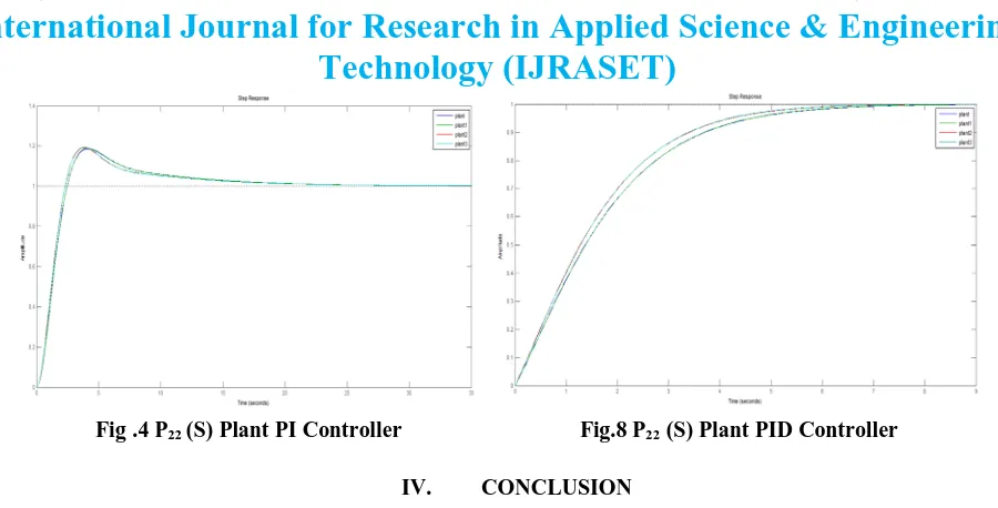
Fig .4 P22 (S) Plant PI Controller Fig.8 P22 (S) Plant PID Controller
IV. CONCLUSION
PI and PID controllers are designed for a given TITO gas turbine application. Similar method can be used for other uncertain systems to design the controller with less computational complexity. PID controller responses are better compared to PI controllers. It has been observed from step responses that PI and PID controller stabilizes the gas turbine system.
REFERENCES
[1]Design of robust PI/PID controller for fuzzy uncertain systems.By B.M patre and R.J Biwani.vol.1no.4,p.p.436-442.2008. [2]Robust control theory and its approach by S.P. Bhattacharya, vol.42,p.p765-771,2012.
[3]Process control and instrumentation by SurekhaBhanoth, vol 47, p.p.324-330.sept-2005.
[4]B. M. Patre and P. J. Deore, “Robust stability and performance for interval process plants,” ISA Transactions, vol. 46, no. 3, pp. 343-349, 2007. [5]B. M.Patre and P. J. Deore, “Robust stabilization of interval plants,” European Control Conference ECC-03, University of Cambridge, Sept. 2003. [6]C. W. Tao, “Robust control of fuzzy systems with fuzzy representation of uncertainties,” Soft Computing,vol. 8, pp.163-172, Springer-Verlag, 2004. [7] C. W. Tao and J. S. Taur, “Robust fuzzy control for a plant with fuzzy linear model,” IEEE Transaction on Fuzzy Systems, vol. 13, pp.30-41, Feb. 2005. [8] H. M. Nehi, “A new ranking method for intuitionistic fuzzy numbers,” International Journal of Fuzzy Systems, vol. 12, no. 1, pp. 80-86, March 2010. [9] H. T. Nguyen, “On foundations of fuzzy theory for soft computing,” International Journal for Fuzzy Systems, vol. 8, no. 1, pp. 39-45, March 2006. [10]D. Driankov, H. Hallendoorn, and M. Reinrank, An Introduction to fuzzy control, Springer, N Y 1993.
[11] D. Dubois and H. Prade, Fuzzy sets and systems: Theory and applications, Academic Press, N Y 1980.
[12] H. T. Nguyen and V. Kreinovich, “How stable is a fuzzy linear system,” Proc. of third IEEE Conference on Fuzzy Systems, pp.1023-1027, June 1994.
[13] H. K. Lam and B. W. K. Ling, “Computational effective stability conditions for time-delay fuzzy systems,” International Journal of Fuzzy Systems, vol. 10, no. 1, pp. 61-70, March 2008.