Statistical Mechanical Framework for Predicting Cellular Response

Response

Thesis by

Lila Forte

In Partial Fulfillment of the Requirements for the degree of

Master of Science

CALIFORNIA INSTITUTE OF TECHNOLOGY

Pasadena, California

©2016

ACKNOWLEDGEMENTS

First and foremost, I would like to express my deepest gratitude to my advisor, Prof.

Tom Miller. His guidance and enthusiasm helped me to overcome many obstacles

during the past two years. I am grateful for all that I have learned from him, the

opportunities I was provided, and the support he has given me. I would also really

like to thank Prof. Justin Bois, not only for the intellectually stimulating conversa-tions and courses, but his tireless attention to his students’ learning and support of

their interests. Also, I would especially like to thank my main collaborator, Connie

Wang. Her support and mentorship were invaluable throughout this process. All the

work done for this thesis would not have been even close to possible without her

extremely patient and insightful guidance. I always enjoyed our conversations and

will miss our strolls and chats. Last, but not least I would like to thank my husband,

ABSTRACT

Developments in singe-cell analysis techniques allow simultaneous high-resolution

measurements of cellular component copy number and variation within a cell

pop-ulation. These data provide a probability distribution for all possible states of the

cell, as determined by the measured component copy number per cell. We have

developed a highly-flexible, theoretical statistical mechanical framework that uses single-cell cellular component data to model the evolution of the probability

distri-bution of those components in a cell in response to an external, physical or

molec-ular, perturbation. This framework uses Bayesian inference to compare potential

functional descriptions of how the perturbation couples to the system, and to

deter-mine the uncertainty in the parameter estimations given the data. We have applied

this methodology to study the impact of changes in oxygen partial pressure on the

behavior of glioblastoma multiform cancer cells. We find that oxygen

concentra-tion couples not only to individual proteins, but effects the underlying effective interactions between the studied proteins as well. The underlying effective interac-tions were found to couple linearly to the system, indicating a simple proportional

change in the protein network across oxygen concentrations. This description of

the system provides improved predictive capabilities for describing the probability

distribution of the measured cellular components across a wider range of

perturba-tion condiperturba-tions than previous methods. Addiperturba-tionally, we apply this methodology

to show how it could be used to predict effects in difficult experimental perturba-tion regimes, identifying undruggable regimes, as well as the result of knocking our

TABLE OF CONTENTS

Acknowledgements . . . iii

Abstract . . . iv

Table of Contents . . . v

List of Illustrations . . . vi

List of Tables . . . viii

Chapter I: Introduction . . . 1

1.1 New Directions Using New Data Collection Methods . . . 1

1.2 Overview . . . 2

1.3 Data: Hypoxia Effect in Cancer Cells . . . 3

Chapter II: Methodology . . . 5

2.1 Theory . . . 5

2.2 Calculations . . . 9

Chapter III: Application: Hypoxia Effect on Cancer Cells . . . 12

3.1 Selection of Perturbation Functional Coupling . . . 12

3.2 Comparison to Previous Analysis . . . 18

3.3 Predictions . . . 22

Chapter IV: Conclusions . . . 27

Bibliography . . . 30

Appendix A: Derivations using Grand Canonical Ensemble . . . 32

A.1 Partition Function . . . 32

A.2 HoEnsemble Statistics . . . 34

LIST OF ILLUSTRATIONS

Number Page

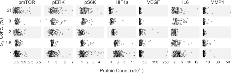
1.1 Measurements of single-cell protein data across tested oxygen

con-centration range. Each dot represents the copy number measured for

that protein in an individual cell. . . 4

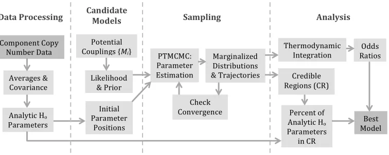
2.1 Workflow for the application of the proposed statistical mechanical

framework to extract from single cell data the best functional

cou-pling of a perturbation to the system. . . 11

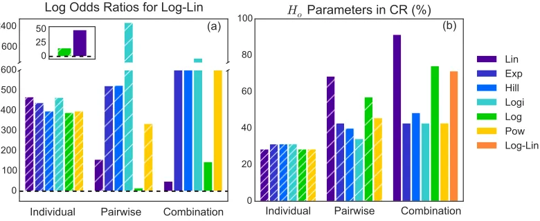
3.1 (a) Positive odds ratios (log shown) for Log-Lin model compared to

all other models indicates is is the most probable model. (b) Percent of analytic Hoparameters, using 21% oxygen as the reference state,

found in the predicted credible regions for those parameters for each

model, indicating that Lin-Lin contains the greatest amount of the

perturbation in the perturbation terms. . . 13

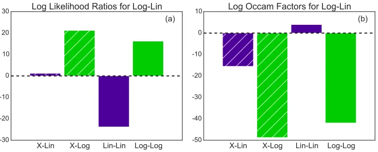
3.2 Estimated contributions to the odds ratio from (a) log likelihood

ra-tios and (b) the Occam factor for the top five models, all in reference

to the Log-Lin model (PLog−Lin/PMi) and calculated using the MAP

parameter values. . . 15

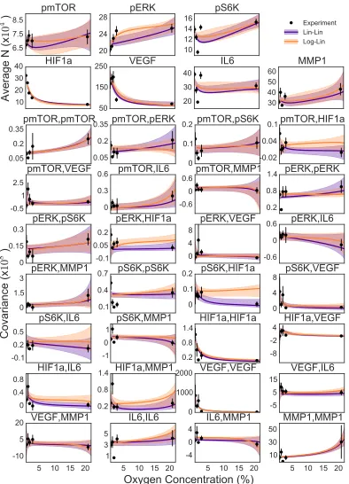
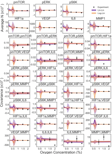
3.3 Fit of Lin-Lin and Log-Lin models to average and covariance in copy

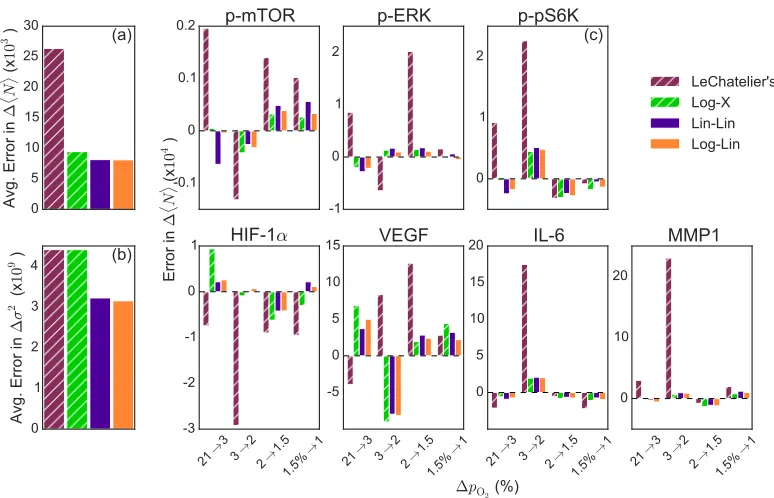
number. . . 17 3.4 Predictions from Log-X, Lin-Lin and Log-Lin models are compared

to quantitative Le Chatelier’s principle model. The average error per

model for predictions of the change in (a) average and (b) covariance

copy number due to a change in oxygen concentration compared to

experimental values. (c) Error per model for predictions in change

in average copy number for each protein. . . 19

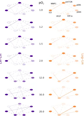
3.5 Protein networks for p-mTOR and VEGF over a range of oxygen

concentrations as predicted by the Log-Lin and Lin-Lin models. Widths

of connecting lines and circles represent strength of effective inter-action, circle fill represents strength of chemical potential. Dashed

3.6 Predictions of average and covariance in copy number with the

Lin-Lin and Log-Lin-Lin models over low oxygen concentrations. . . 23

3.7 Predictions from Log-Lin model showing effects of removing re-moving the effective interaction between pmTOR and pERK. . . 25 3.8 Predictions from Log-Lin model showing effects of knocking out

pmTOR. . . 26

B.1 Walker trajectories for 200 walkers are shown. The average value is

shown in red. Three of 42 parameters are shown for the Lin-X model. 39

LIST OF TABLES

Number Page

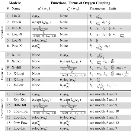
2.1 Proposed functional forms of oxygen coupling. . . 7

C h a p t e r 1

INTRODUCTION

1.1 New Directions Using New Data Collection Methods

With advances in quantitative single-cell analysis techniques, we now have the

abil-ity to observe the steady-state probabilabil-ity distribution for copy number of most cel-lular components (e.g. proteins, mRNAs, metabolites, etc.) under specific

condi-tions. This distribution contains information beyond population averages,

describ-ing the effective interactions between multiple cellular components, however the challenge is how to extract this information. The steady-state that can be obtained

is defined by nearly constant average concentration of a cellular component over

time after the application of a stimulus and given time to relax in those conditions.

Following a perturbation, such as the addition of a drug or changes in resources

available, cells may come to a different steady-state than before the stimulus was applied [1]. Novel technologies now exist that can measure simultaneous cellular component copy numbers to obtain the multi-dimensional steady state probability

distribution over a range of perturbation conditions [2].

Stochasticity in gene expression, due to intrinsic and extrinsic noise [3], gives rise

to fluctuations in protein levels and causes clonal populations of cells to exhibit

phenotypic variation at steady state [1, 4, 5]. The steady-state distribution of cellular

component copy number for an ensemble of genetically identical cells provides the

most probable copy numbers (average), as well as fluctuations in copy number for cells in the population. The noise in expression levels of cellular components, or

fluctuations in a population, have been associated with drug resistance, variation in

cell-to-cell response to external stress and cell differentiation [4, 6–8]. Therefore, a clear understanding of the steady-state copy number distribution would help to

predict when and what response may occur due to an external stimuli.

Master equation formulations, which use known parameters for rates of

produc-tion and diluproduc-tion due to cell division, have been used to predict the steady state

distribution for individual cellular components for a population of cells and then checked with single cell analysis at one set of experimental conditions [9–11]. An

inverted method can obtain parameters given a steady state distribution under one

Therefore, understanding how the steady state distribution is coupled to a

perturba-tion will give more informaperturba-tion on dynamics of the system in response to that

per-turbation. However, since it is often experimentally intractable to take single-cell measurements of every possible perturbation condition, we instead obtain

“snap-shots” under specific external conditions. The challenge is to extract from those few

measurements, how the steady-state distribution evolves as a function of a specific

perturbation, such as changing the concentration of a drug or steadily decreasing

cellular resources.

Specifically, we are interested in extracting from the few isolated experimental

mea-surements how the copy number in a cell, that is the probability distribution of the

number density, evolves as a perturbation is increased or decreased. In some fam-ilies of active matter systems, thermodynamic equilibrium approaches have been

used, taking a number density view of the system [12, 13]. Homogeneous steady

states have been seen in active matter systems to arise from the effective generation of long-range interactions in the system, even if local density variations are ignored

[14]. We therefore approach the system from a thermal equilibrium perspective,

where the “free energy” of the system is relative to the number density for each

cel-lular component in the cell. We are not concerned with the mechanistic or physical

interactions of the proteins, but instead how the effective interactions and funda-mental characteristics of the measured proteins, captured in the single cell data, evolve as a function of the perturbation.

1.2 Overview

We apply an equilibrium statistical mechanical framework to model the evolution of

the probability distribution of cellular components in a cell in response to an

exter-nal perturbation. We use the number density for each cellular component to define

the state of the cell. Each cellular component interacts with every other measured

cellular component with an associated interaction energy, providing an effective long-range interaction among the components. Additionally, the individual

proper-ties, that is the chemical potentials, for each cellular component determine the total

energetics for the cell. The stable, grand canonical statistical distribution for a pop-ulation of clonal cells describes the possible states of these cells in the poppop-ulation,

as determined by their volume, temperature and internal properties or interactions,

and contains information on the average and fluctuations of those cellular

compo-nents. We propose simple Hamiltonian forms that describe the functional coupling

ex-tract the best available parameterization using Bayesian inference. The functional

coupling can be utilized to predict properties of the effective protein interaction network as a function of the perturbation.

1.3 Data: Hypoxia Effect in Cancer Cells

We apply our methodology to a data set describing the effect of hypoxia on cancer cells. In the center of most tumors, particularly in solid organ cancers, hypoxic

conditions with oxygen partial pressures _. 3% pO2 arise due to rapid cell growth,

constriction or leaking of blood vessels, increased interstitial pressure, or edema[15,

16]. The cancer cells in these hypoxic micro environments change their metabolism

through HIF and mTOR signaling pathways in order to survive [17]. Tumors with

hypoxic conditions can exhibit increased proliferation, aggression, and even a

de-crease in response to drug therapies[18, 19].

The molecular mechanisms in this system are well known, but the quantitative

ef-fects of oxygen on these signaling networks are less clear. Heathet. al. performed an experimental study of the mTOR and HIF signaling networks using single-cell

barcode chip (SCBC) techniques [19]. We apply our statistical mechanical

frame-work to their data set to investigate the effect of changes in the oxygen partial pres-sure on protein signaling networks in glioblastoma multiform (GBM) cancer cells.

The SCBC method is a microfluidics platform that quantifies a panel of proteins

from statistical numbers of single cells [2]. For this experiment, cells are loaded into chambers on a microchip, about 1 cell/microchamber. The cells on the chip are incubated at a specific oxygen concentration for 7 hr. The cells are then lysed, and

secreted and intracellular proteins are captured using an antibody mixture with

flu-orescent probes. Copy numbers for each protein are inferred from the fluorescence

intensity of each micro chamber. For this experiment, seven key functional proteins

in the HIF and mTOR signaling pathways were chosen for the panel and single-cell

data was collected at 21%, 3%, 2%, 1.5%, and 1% pO2. Under each oxygen

condi-tion, ~100 single cells were analyzed, providing protein copy number data per cell

0.5 1.5 2.5 3.5

21

3

2

1.5

1 O2

C

on

c.

(%

)

pmTOR

1 3 5 7

pERK

1 2 3 4

pS6K

1 3 5 7

Protein Count (x104₎

HIF1a

50 150 250

VEGF

2 6 10 12

IL6

10 30 50

[image:12.612.112.505.76.200.2]

MMP1

Figure 1.1: Measurements of single-cell protein data across tested oxygen

concen-tration range. Each dot represents the copy number measured for that protein in an

C h a p t e r 2

METHODOLOGY

2.1 Theory

We define a Hamiltonian for an n-component system, which is a function of the copy number, Ni, of each component, i and the perturbation, λ. We consider the

state of a cell can be fully described by the copy number of its components.

H({Ni}, λ) = Ho({Ni})+H1({Ni}, λ) (2.1)

The first term, Ho, is a reference state Hamiltonian that describes the system in

absence of the perturbation, while H1 contains the physics that describes how the

perturbation functionally couples to the system. With no prior knowledge as to the

functional form of H1, this methodology provides a framework in which to extract

this information from the data.

The reference state Hamiltonian for ann-component system is defined as

Ho({Ni}) = n

X

i,i≥j

αi jNiNj − n

X

i

µiNi (2.2)

where µi is the chemical potential for componentiandαi j is the effective pairwise

interaction between componentsiand j. Assuming a well mixed solution, such that the density of each cellular component, ρi, is uniform across the cell with a constant

volume,V,

Ho({ρi})= n

X

i,i≥j

ai jρiρjV − n

X

i

µiρiV (2.3)

whereai j = αi jV, such thatai j has units _NV2 and µi has units

N, and is an energy

unit. The effective pairwise interaction parameters, {ai j}, describe the network of

protein interactions, but provide no information on mechanistic or physical

inter-actions. The parameters inHodescribe the fundamental interactions and potentials

for the set of cellular components under the reference state conditions.

The functional coupling of a physical external perturbation to the system,H1, such

as addition of a drug or changes in cellular resources, is defined as

H1({Ni}, λ) = n

X

i,i≥j

fi j(λ)

V NiNj−

n

X

i

where the perturbation terms, fi j(λ) andgi(λ), describe how the perturbation changes

the effective pairwise interactions for each pair of components and chemical poten-tials for each cellular component, respectively. Additionally, fi j(λ) andgi(λ) are

zero at the reference state conditions (λo), so that under the specified external

con-ditions,H({Ni}, λo)= Ho({Ni}). Due to the form of the Hamiltonian,H, the choice

of reference state conditions is mathematically arbitrary. Any choice ofλoprovides

identical information on the functional coupling to the perturbation, H1, the only

difference begging that the information on the fundamental interactions and poten-tials are for that chosen reference state, Ho.

We apply this framework to study the effects of hypoxic conditions on glioblastoma multiform cancer cells. We choose a set of candidate hamiltonians, {H1}, that

de-scribe possible simple functional couplings of oxygen concentration to the system

(Table 2.1). As the effective coupling of oxygen to these proteins is unknown, we begin with simple functions commonly seen in biological systems. Additionally,

we include three levels of coupling: individual, pairwise, and a combination of the

two. We define the reference state as normoxic conditions, 21% oxygen

concentra-tion such that the perturbaconcentra-tions is zero at p21, according to

gi(pO2) =gi∗(pO2)−gi∗(p21) (2.5)

fi j(pO2) = f

∗

i j(pO2)− f

∗

i j(p21) (2.6)

whereg_i∗(pO2) and fi j∗(pO2) contain the functional coupling of oxygen

concentra-tion to the system, and g_i∗(p21) and fi j∗(p21) have the same functional forms and

parameters asg_i∗(pO2) and fi j∗(pO2), respectively, but are evaluated at only the

Models: Functional Forms of Oxygen Coupling

# : Name g_i∗ pO2

f_{i j}∗ pO2

Parameters : Units

1 : Lin-X kipO2 None ki : _{N p}

O2

2 : Exp-X biexp(kipO2) None ki : _p1

O2 bi :

N

3 : Hill-X bi

1+(ki/p_O2)mi None ki : pO2 bi :

N mi:−

4 : Logi-X bi

1+exp[−mi(p_O2−ki)] None ki : pO2 bi :

N mi:

1

p_O2

Indi

vidual

5 : Log-X bilog(pO2) None bi : _N

6 : Pow-X bip_Omi

2 None bi :

N pmi

O2

mi :−

7 : X-Lin None ki jpO2 ki j : _N2V_p O2

8 : X-Exp None bi jexp(ki jpO2) ki j : 1

p_O2 bi j :

V N2

9 : X-Hill None _1+(k bi j

i j/p_O2)mi ki j : pO2 bi j :

V

N2 mi j :−

10 : X-Logi None bi j

1+exp[−mi j(p_O2−ki j)] ki j : pO2 bi j :

V N2 mi j :

1

p_O2

P

airwise

11 : X-Log None bi jlog(pO2) bi j :

V N2

12 : X-Pow None bi jp mi j

O2 bi j :

V N2_pmi

O2

mi j :−

13 : Lin-Lin kipO2 ki jpO2 see models 1 and 7

14 : Exp-Exp biexp(kipO2) bi jexp(ki jpO2) see models 2 and 8

15 : Hill-Hill bi

1+(ki/p_O2)mi

bi j

1+(ki j/p_O2)mi see models 3 and 9

16 : Logi-Logi bi

1+exp[−mi(p_O2−ki)]

b_{i j}

1+exp[−mi j(p_O2−ki j)] see models 4 and 10

Combination _{17 : Log-Log bilog(pO}

2) bi jlog(pO2) see models 5 and 11

18 : Pow-Pow bip_O2mi bi jp mi j

O2 see models 6 and 12

[image:15.612.91.525.71.507.2]

19 : Log-Lin bilog(pO2) ki jpO2 see models 5 and 7

Table 2.1: Proposed functional forms of oxygen coupling.

The grand canonical partition function,Ξ, for ann-component system is defined as

Ξ(β,V,{µ_i},{ai j},{gi(λ)},{fi j(λ)}) =

∞

X

N1=0

∞

X

N2=0

. . . ∞

X

Nn=0

e−βH(λ,N1,N2,...,Nn) _(2.7)

where β = 1/kBT, andkB is the Boltzmann constant. The discrete partition

func-tion is not analytically solvable, but we can approximate the partifunc-tion funcfunc-tion as a

continuous integral over all possiblen-component densities, which is exactly solv-able (see Appendix A.1 for full derivation of the partition function). The analytic

Ξ(β,V,{µi},{ai j},{gi(λ)},{fi j(λ)})= * ,

V√2π 2 +

-n

e12(M+G)T(A+F)

−1_(M+G)

√

|A+F| (2.8)

where

(M+G)T = βV µ₁+g1(λ) µ2+g2(λ) . . . µn+gn(λ)

A+F=2βV

* . . . . . . .

,

a11+ f11(λ) 1₂(a12+ f12(λ)) . . . 1₂(a1n+ f1n(λ))

1

2(a21+ f21(λ)) a22+ f22(λ) . . . 1

2(a2n+ f2n(λ))

... ... . . . ...

1

2(an1+ fn1(λ))

1

2(an2+ fn2(λ)) . . . ann+ fnn + / / / / / / /

-such that A+F is a symmetric matrix, for which (A+F)−1 and |A+F| are the inverse and determinant, respectively.

Importantly, the analytic partition function contains all of the information about

the statistical distribution for cellular component copy numbers. Two observable

thermodynamic properties describing the ensemble behavior, the average,hNii, and

fluctuations,h(δNi)(δNj)i, of the cellular component copy number, can be derived

from this partition function. Evaluation of the first and second derivatives of the

partition function, with respect to the conjugate thermodynamic quantity to particle

number,−β µ, provides predictions for the mean and covariance in cellular

compo-nent copy number

hNii=V

X

j

(µj+gj(λ))(ai j+ fi j(λ))−1 (2.9)

h(δNi)(δNj)i= σi j =

V

β(ai j + fi j(λ))−1 (2.10)

where (ai j+ fi j(λ))−1is an element of the inverseA+Fmatrix (see Appendix A.2

for then-component derivation). These equations show directly how the perturba-tion affects each observable moment of the steady state probability distribution.

Not only do Eq. 2.9 and Eq. 2.10 provide simple relations of the statistical

behav-iors and the perturbation, when no perturbation is applied, at the reference state,

hNii=V

X

j

µjai j−1 (2.11)

σi j =

V

βa−i j1 (2.12)

wherea−_{i j}1is an element inA−1. There is a clear 1-to-1 mapping of experimentally observed statistics (i.e. hNiito parameter values (i.e. µi). These statistics, average

and covariance in cellular component copy number, can be easily measured with

single cell analysis techniques. Therefore, through inversion of Eq. 2.11 and Eq.

2.12, we derive the unique natural parameter values for the chosen reference state

from experimental data collected under those conditions

µi = β−1

X

j

hNjiσi j−1 (2.13)

aii =

V 2βσ

−1

ii (2.14)

ai j =

V βσ

−1

i j (2.15)

whereσ−_{i j}1is an element of the inverse covariance matrix.

However, to fully understand the perturbation coupling we must obtain the

param-eters in the perturbation coupling terms, gi(λ) and fi j(λ). Due to the additional

parameters present in these terms, the full Hamiltonian system is underdetermined.

There is no unique analytical solutions for the parameters derived directly from

ex-perimental quantities as was conveniently possible with Ho. Therefore, we utilize

Bayesian inference to systematically obtain best fit parameters for each candidate

Hamiltonian form of coupling of the perturbation to the system, and extract from

the data the proper functional coupling of the perturbation to our system.

2.2 Calculations

From an experimental data set, D, containingn-component copy numbers from in-dividual cells over a range of perturbation conditions, we apply Bayesian inference

to acquire the most probable functional perturbation coupling and parameterization.

The probability of each candidate Hamiltonian (Table 2.1), or model, is evaluated

(PTMCMC) is used to efficiently sample the high-dimensional parameter sets for each model.

We use PTMCMC, for each model, Mi, to sample the posterior distribution

asso-ciated with the parameter set, γi, for model i, where γi contains {ai j}, {µi} and

any parameters contained in the coupling terms, {fi j(λ)} and {gi(λ)}. According

to Bayes’ theorem, the posterior distribution for the parameter set, P(γi|D,Mi), is

proportional to the likelihood, P(D|γ_i,Mi), times the prior probability, P(γi|Mi).

The likelihood, or the probability of the data given Mi, is defined by a Boltzmann

distribution

P(D|γi,Mi) =

1

Ξi(β,V, γi,Mi)

e−βHi(D) _(2.16)

where Hi and Ξi are the Hamiltonian and partition function for modeli. For the

prior probability, each of them-parameters inγiis considered independent. We use

an uninformative, uniform prior for each individual parameter over a broad range

of values

P(γi|Mi) = m

Y

j=1

P(γi,j|Mi)= m

Y

j=1

1 γmax

i,j −γ min i,j

(2.17)

where γ_imax_,j and γ_imin_,j define the range allowed for parameter γi,j (see Appendix

B for full ranges of parameter values used for each model). For the sampling,

parameters are initialized within this range, and we use the data from the reference

state conditions and Eqs. 2.13-2.15 to find a reasonable parameter space to initialize

{ai j} and {µi}and any parameters in {fi j(λ)} and {gi(λ)} such that the change in {ai j}and{µi}is small to keep the values in physically reasonable ranges initially.

The EMCEE package [20, 21] is used to perform the PTMCMC calculations. Each

calculation is run with 20 temperatures, 2,000 walkers for 8,000-10,000 steps until

convergence is reached (see Appendix B for convergence criteria discussion). We

then obtain the most probable values (modes) and 95% credible regions for each

parameter estimate using the marginalized distribution for the lowest temperature

PTMCMC.

By sampling many temperatures, we are able to calculate the odds ratio,Oi j, which

we use to compare modelsi and j,

Oi j =

P(Mi|D)

P(Mj|D) =

P(Mi)P(D|Mi)

P(Mj)P(D|Mj) =

R

dγiP(γi|Mi)P(D|γi,Mi)

R

dγjP(γj|Mj)P(D|γj,Mj)

(2.18)

We assumea priorithat all models are equally likely, P(Mi) = P(Mj). This form

for each temperature,B, sampled in the PTMCMC we calculate

Zi(B)=

Z

dγiP(γi|Mi)[P(D|γi,Mi)]B (2.19)

Then we use thermodynamic integration to find

lnP(D|Mi) =ln Zi(1)=

Z 1

0

dBhln[P(D|γi,Mi)]iB (2.20)

According to Bayes’ theorem, the calculation of the odds ratio allows us to deter-mine which tested model is most probable given the experimental data. To provide

information on how close to an “ideal” model we are, that is have we tested enough

models, we propose a metric to quantify the amount of perturbation captured by

our perturbation terms, {gi(λ)} and {fi j(λ)}, for each model. For this calculation,

we check if the analytic reference state parameters found by solving Eqs. 2.13-2.15

for Ho are found within the predicted credible regions from Bayesian analysis for

those parameters. We assume that for an ideal model, where all of the perturbation

effects on copy number are captured by the perturbation terms, 100% of the ana-lytic parameters from Ho will fall into the predicted credible regions. Our entire

[image:19.612.121.499.440.591.2]

workflow to determine the functional form of the perturbation coupling is shown in

Figure 2.1.

Data Processing Sampling Analysis

Component Copy Number Data

Averages & Covariance

Analytic Ho

Parameters

Potential Couplings {Mi}

Likelihood & Prior

PTMCMC: Parameter Estimation

Initial Parameter

Positions

Check Convergence

Thermodynamic Integration

Credible Regions (CR) Marginalized

Distributions & Trajectories

Odds Ratios

Percent of Analytic Ho

Parameters in CR

Best Model Candidate

Models

Figure 2.1: Workflow for the application of the proposed statistical mechanical

framework to extract from single cell data the best functional coupling of a

C h a p t e r 3

APPLICATION: HYPOXIA EFFECT ON CANCER CELLS

We utilize our statistical mechanical framework to analyze the effect of changing oxygen partial pressure on GBM cancer cells. We use this workflow to extract the

functional coupling of oxygen to the steady state distribution of copy number for

seven measured proteins from the single-cell data. This functional coupling can

then be used to make predict copy number distributions under varying conditions.

These predictions have several useful applications, including identification of un-druggable regimes or potential drug targets in complex protein networks.

3.1 Selection of Perturbation Functional Coupling

To determine the functional coupling of oxygen to the steady state probability

dis-tribution for the seven measured proteins in our data set, we define 19 candidate

Hamiltonians. We are interested in identifying the most simple coupling that can

describe the system, so our first six Hamiltonians only have couplings of oxygen

to individual proteins, i.e. gi(pO2) only (Table 2.1 : M1− M6). Biologically, this

indicates that there are a set of fundamental effective protein interactions, which remain unchanged due to changes in oxygen. These models have direct

connec-tions to a previous analysis done by Heath et. al using a quantitative Le Chatelier’s

model[19], but contain more information about the functional form of the coupling to the individual proteins. The next six models contain couplings to the effective interactions between pairs of proteins (fi j(pO2)) only (Table 2.1 : M7− M12). The

final seven models are a set of Hamiltonians that are combinations of the pairwise

and individual couplings (Table 2.1 : M13−M19). For all models, the reference state

chosen is at 21% pO2, since this is the concentration most typically used inin-vitro

studies.

The functional forms for these models were chosen for their simplicity or

similar-ity to common functional forms seen in biological systems. We analyze a simple

linear coupling indicating a constant proportional relationship between changes in

oxygen and protein concentration. Additionally we look at three functions,

expo-nential, logarithmic, and a general power function, indicating that the oxygen

indicate protein production or interactions may change at some threshold oxygen

concentration. To determine the probability of each of these functional couplings,

we analyze the odds ratios (only the odds ratios for the Log-Lin model are shown in Fig. 3.1a), and what percent of the perturbation is captured by each model using

our afore mentioned metic (Fig. 3.1b).

1600 2400

Individual Pairwise Combination (a)

Log Odds Ratios for Log-Lin

0 100 200 300 400 500 600

0 20 40 60 80 100

Individual Pairwise Combination (b) H_o

Parameters in CR (%)

Lin Exp Hill Logi Log Pow Log-Lin

[image:21.612.114.504.176.336.2]

0 25 50

Figure 3.1: (a) Positive odds ratios (log shown) for Log-Lin model compared to

all other models indicates is is the most probable model. (b) Percent of analyticHo

parameters, using 21% oxygen as the reference state, found in the predicted credible

regions for those parameters for each model, indicating that Lin-Lin contains the greatest amount of the perturbation in the perturbation terms.

Overall, oxygen couplings to individual proteins only, that is with no effect on the protein interactions or network, have similar, low probabilities (Fig.3.1a) and

cap-ture the least of the perturbation (Fig.3.1b), irrespective of the functional form of the

coupling. This indicates that hypoxic conditions, or oxygen perturbations, affect not only the average copy number, but the fluctuations as well. Therefore, the effective protein interaction network is likely altered under varying oxygen conditions.

In general, two functional forms, logarithmic and linear oxygen coupling are

su-perior to the other switching, exponential or power functional couplings. This is

seen both when the coupling occurs in only a pairwise manner or in a

combina-tion of pairwise and individual protein couplings. These funccombina-tional forms, seen

in the X-Lin, X-Log, Lin-Lin, Log-Log, and Log-Lin models, are not only most

likely overall, but also capture the greatest amount of perturbation compared to all

models, all containing over 50% of the perturbation. Interestingly, at low oxygen

much of our data is in this low oxygen range, that is four out of the five

experimen-tal conditions were ≤ 3%pO2, all five of these models agree that the perturbation

effect is linear in low oxygen regimes.

According to the odds ratio, the Log-Linear (M19) model is most probable given

the fit and complexity of the models tested for this data (Fig.3.1a). The next best

two models are X-Log (M11) and Lin-Lin (M13), but are significantly (> e10) less

probable. However, our metric describing the percent of the perturbation captured

by a model (Fig 3.1b), indicates that the Lin-Lin model captures 91% of the

pertur-bation, while X-Log and Log-Lin only capture 54% and 71% of the perturpertur-bation,

respectively. This metric suggests that the Lin-Lin model best describes the

intrin-sic parameter set for the reference state, and may be close to an ideal model, which is in disagreement with the odds ratio.

Since the odds ratio is an unbiased metric, derived directly from Bayes’ theorem

with no approximations, the Log-Lin model is likely the best model we have tested.

However, the discrepancy that arises from the Lin-Lin model capturing over 20%

more of the perturbation than any other model, begs the question of what makes

the Log-Lin model so much more probable. Therefore, we examine the two

com-ponents that make up the odds ratio, the goodness of fit of the model to the data and the complexity of the model. The contributions of these two properties can be

estimated using the likelihood ratio and the Occam factor for each pair of models,

giving insight into the ordering of the odds ratios.

To estimates the posterior distribution we approximate the distribution as gaussian

and compare the relative hight and width of the distributions for each model. The

likelihood ratio compares the goodness of fit, or the height of the posterior, between

two models. The likelihood is the probability at the maximum a posteriori (MAP).

Using the most probable parameter set, the likelihood is calculated from our pa-rameter estimation (P(D|Mi, γ_iMAP)). The Occam factor penalizes more complex

models, those with more parameters, as well as models with less flexibility, that is

models having less parameter values consistent with a given model. The Occam

factor can be estimated by comparing the ratios of the widths of the priors to the

widths of the posterior distributions [24],

Occam Factor Mi Mj

!

= P({γ}|Mj) Qn

k=1C R(γk)i

P({γ}|Mi)Qn_k=1C R(γk)j

(3.1)

reference since it is the most probable model overall. We only examine the top five

models in this analysis.

X-Lin X-Log Lin-Lin Log-Log

-30 -20 -10 0 10 20 30

(a)

Log Likelihood Ratios for Log-Lin

X-Lin X-Log Lin-Lin Log-Log

-50 -40 -30 -20 -10 0 10

[image:23.612.112.500.124.280.2]

(b)

Log Occam Factors for Log-Lin

Figure 3.2: Estimated contributions to the odds ratio from (a) log likelihood ratios

and (b) the Occam factor for the top five models, all in reference to the Log-Lin

model (PLog−Lin/PMi) and calculated using the MAP parameter values.

Investigation into the likelihood ratio indicates that the Lin-Lin model has a much

better fit (> e20) than the Log-Lin model, and that the X-Lin model has a nearly identical fit to the Log-Lin model. This agrees with the metic determining the per-cent of perturbation captured, indicating that metric is dependent on the fit of the

model. Lin-Lin being the best fit explains that this model likely has less of the

per-turbation overflow into the intrinsic parameter set for the reference state during the

parameter search, and why it has such a high percent of the perturbation captured

in the proper terms. Additionally, this analysis implies that the models with linear

functional coupling in the pairwise terms best fit this data set, indicating a linear

relation between oxygen concentration and effective protein interactions.

However, the Occam factor analysis illustrates that the Lin-Lin model is penalized

because it is more complex than the X-Lin and X-Log models, having seven more

parameters. Additionally, the Occam factors suggest that the logarithmic functional

form provides greater flexibility in the number of possible parameters that have the

same probability in the model, increasing the overall probability of the model, as

functions with this form have better Occam factors (Fig. 3.2b). It is also clear that

the X-Log model is the second most probable model overall, even though it has a

Lin-Lin or Log-Lin) and the increased flexibility due to the logarithmic functional

coupling.

Overall, the logarithmic terms seem to add flexibility, but decrease the fit of the

model. This may be due to there being some leveling offof copy number or fluc-tuations at higher oxygen concentrations. Even if the lower oxygen concentrations

seem to fit a more linear model, the high oxygen concentration copy numbers could

limit the number of parameters in a linear model that fit the data equally well.

Therefore, the Lin-Lin model, even though it has a high fit for this data set, would

be too inflexible and make poor predictions for further experiments. The greater

range of parameter values allowed by the logarithmic terms in the Log-Lin model

indicate that this model will likely make better predictions over a greater range of oxygen concentrations.

The relative fit and flexibility of these two models can also be compared visually

(Fig. 3.3). Although we see larger credible regions for the Log-Lin model,

indicat-ing greater flexibility but also an indication of a worse fit. Overall, the two models

are quite similar. Without more data it would be difficult to distinguish if the Lin-Lin model is overfit for this dataset, or if it actually is a more accurate representation

of natural functional coupling of oxygen to this system of proteins.

Biologically, the functional forms for both the top models, Lin-Lin and Log-Lin,

indicate that the oxygen causes a linear response in the effective protein interaction network. The results also show that the pairwise interactions changing is likely a

key aspect of the system’s response to a perturbation. Surprisingly, even though

the perturbation is linear in each effective protein pair interaction, the fluctuations and covariance change can be much more complex due to the many interacting

pro-teins (Fig. 3.3). There is however still some ambiguity about whether the chemical

potentials couple linearly or logarithmically to the oxygen concentration. More ex-perimentation would be useful to distinguish this coupling, particularly at a few

more oxygen concentrations, perhaps 10% and 80% pO2 to get a full range of

be-haviors. Due to this uncertainty, for the rest of the analysis, both the Lin-Lin and

6.5 7.5 8.5

pmTOR

20 24 28

pERK

10 12 14 16

pS6K

10 20 30 40

A

ve

ra

ge

N

(x

10

4

)

HIF1a

50 150 250

VEGF

20 30 40

IL6

30 40 50 60

MMP1

Experiment Lin-Lin Log-Lin 0.05 0.2 0.35

pmTOR,pmTOR

0.05 0.2 0.35

pmTOR,pERK

0 0.1 0.2

pmTOR,pS6K

-0.02 0.04 0.1

pmTOR,HIF1a

-0.5 1 2.5

pmTOR,VEGF

0 0.3 0.6

pmTOR,IL6

-0.6 0 0.6

pmTOR,MMP1

0.2 0.8 1.4

pERK,pERK

0 0.15 0.3

pERK,pS6K

-0.1 0.05 0.2

pERK,HIF1a

0 4 8

pERK,VEGF

-0.6 0 0.6

pERK,IL6

0 1.5 3

C

ov

ar

ia

nc

e

(x

10

8

)

pERK,MMP1

0.1 0.4 0.7

pS6K,pS6K

0 0.1 0.2

pS6K,HIF1a

0 4 8

pS6K,VEGF

-0.1 0.2 0.5

pS6K,IL6

-1 0 1

pS6K,MMP1

0.2 0.8 1.4

HIF1a,HIF1a

-8 -2 4

HIF1a,VEGF

0 0.4 0.8

HIF1a,IL6

0.2 0.8 1.4

HIF1a,MMP1

0 1000 2000

VEGF,VEGF

-5 5 15

VEGF,IL6

5 10 15 20 -10

5

20

VEGF,MMP1

5 10 15 20

Oxygen Concentration (%)

1 3 5

IL6,IL6

5 10 15 20 -4

0 4

IL6,MMP1

5 10 15 20 10

30 50

[image:25.612.111.505.70.616.2]

MMP1,MMP1

Figure 3.3: Fit of Lin-Lin and Log-Lin models to average and covariance in copy

3.2 Comparison to Previous Analysis

We compare our framework and models to a previous analysis of this data, which

used a quantitative version of Le Chatelier’s principle[19]. The Le Chatelier’s

prin-ciple model relates the change in average copy number with a change in the

chem-ical potentials due to a change in the external conditions, but does not specify the

form of the change in chemical potentials over oxygen ranges. This model assumes

constant fluctuations (or covariance), which is analogous to our models with only

individual protein couplings (M1−M7). However, even with these simple models

we have the ability to identify the specific functional form of the perturbation,

un-like the Le Chatelier’s principle model, which means we can predict copy number

averages and covariances, where as the Le Chatelier’s principle can only predict a

change.

To analyze what information is gained by the addition of the functional form we

compare our most probable model from the first six models, Log-X, to Le

Chate-lier’s principle model. Additionally, to see what is lost by assuming the fluctuations are constant, and how that effects our predictive capabilities, we compare our best fitting models, Log-Lin and Lin-Lin, to the Le Chatelier’s principle model. Since

the Le Chatelier’s principle model can only predict changes in average copy

num-ber and predicts no changes in covariance, we analyze the error in these predictions

compared to experiment for each model overall (Fig 3.4a-b) and by protein (Fig

0 5 10 15 20 25 30

Avg. Error in

∆

­ N ® (x

10

3) (a)

0 1 2 3 4

Avg. Error in

∆

σ

2 (x

10

9) (b)

-0.1 0 0.1 0.2

p-mTOR

-1 0 1 2

p-ERK

0 1 2 (c)

p-pS6K

21→ 3

3→2

2→1.5

1.5% →1 -3 -2 -1 0 1 Error in ∆ ­ N ® (x

10

4)

HIF-1

α

21→

3

3→2

2→1.5

1.5%

→1

∆pO2 (%) -5 0 5 10 15

VEGF

21→ 3

3→2

2→1.5

1.5% →1 0 5 10 15 20

IL-6

21→ 3

3→2

2→1.5

[image:27.612.115.502.69.318.2]

1.5% →1 0 10 20

MMP1

LeChatelier's Log-X Lin-Lin Log-Lin

Figure 3.4: Predictions from Log-X, Lin-Lin and Log-Lin models are compared to quantitative Le Chatelier’s principle model. The average error per model for

predictions of the change in (a) average and (b) covariance copy number due to

a change in oxygen concentration compared to experimental values. (c) Error per

model for predictions in change in average copy number for each protein.

Overall, our top models are significantly more accurate, at least two times more so,

than the previous Le Chatelier’s principle model in predicting the change in average

copy number (Fig. 3.4a). Log-X, like Le Chatelier’s principle, assumes constant

effective protein interactions and therefore has constant covariance, so we see the same poor prediction in covariance change (Fig.3.4b). However, the Log-X

com-parison shows that just knowing the functional form provides increased predictive

capabilities for change in copy number. The functional form implies that the growth

rates of proteins may be effected by changes in oxygen concentration in a logarith-mic fashion. We again see that Lin-Lin and Log-Lin are similar, and both are more

accurate at fitting both, average and covariance, than models with no pairwise

cou-pling (Log-X or Le Chatelier’s). However, Log-Lin is actually better at predicting

changes in covariance than Lin-Lin, perhaps another indication of its being the most

probable model, and increasing the evidence that the individual protein growth rates are affected logarithmically by oxygen change.

makes poor predictions for some particular ranges in oxygen, particularly from 3%

to 2% pO2. Our models however, have more consistent error across all oxygen

changes, overall fitting the data more accurately, and increasing our confidence in more expansive predictive capabilities of the model. Additionally, by looking over

the individual proteins, some models, including Le Chatelier’s, do better, sometimes

significantly so, for one protein and very poorly for another. This could indicate

that mixed models, where each protein could have a different type of individual or pairwise functional form may provide even more actuate models.

The poor predictions using Le Chatelier’s principle model between 3% and 2%

pO2 were attributed to the oxygen concentration being a strong perturbation in this

regime, which was considered the cause for the disagreement with the theory[19]. Our model does not support this, and therefore see no reason to assume one

concen-tration is a stronger or weaker perturbation, but instead the effect seen is due to the functional coupling of the oxygen concentration to the system. Additionally, using

PCA analysis, the previous model indicated that a few proteins became decoupled

from the network. Specifically, VEGF seemed to be unpredictable between 2% and

1.5% pO2, perhaps decoupling from the rest of the network. There also seemed to

be a loss in mTOR signaling coordination, which lead to p-mTOR becoming

unre-sponsive to some drug treatments[19]. However, they were unable to specifically

[image:29.612.164.451.72.466.2]

Figure 3.5: Protein networks for p-mTOR and VEGF over a range of oxygen con-centrations as predicted by the Log-Lin and Lin-Lin models. Widths of

connect-ing lines and circles represent strength of effective interaction, circle fill represents strength of chemical potential. Dashed and solid lines represent inverse and positive

effective pairwise interactions, respectively.

Both of our best fit models indicate that VEGF does indeed become decoupled, and

then changes sign of interaction with p-ERK, HIF-1α, IL6 and itself, between 1%

and 2% pO2 (Fig. 3.5). Additionally, the chemical potential of VEGF also goes to

zero, though at 2% pO2 in the Lin-Lin model and 1% pO2 in the Log-Lin model.

The chemical potential gives us an indication of the natural flux in copy number,

and therefore, in this range there could be large fluctuations in the particle number

possible, which is in agreement with what the previous analysis saw for this protein.

However, unlike in the Le Chatelier’s principle model, p-mTOR does not seem to

have a loss in its signaling network between 1.5-2% pO2. There is a slight

weaken-ing of the interactions from p-mTOR to all other proteins as oxygen concentration

increases. However the protein network only becomes significantly different for mTOR at high oxygen concentrations (12-20 pO2), which is wherein-vitrostudies

are conducted. In order to test the validity of these predictions in the protein

signal-ing network, ssignal-ingle-cell data at more oxygen concentrations between 21% and 3%

would be useful.

From this analysis, we see that our framework provides a more specific picture

of system’s response to a perturbation. We are able to examine not just a change

in copy number, but also specific network and individual protein characteristics,

providing more insight into the biological response.

3.3 Predictions

Besides gaining information on the functional coupling of the perturbation to the

system, this framework can also make predictions outside of the measured

pertur-bation conditions or related to testable changes to the protein network, such as the

knocking out a protein or an interaction.

Predictions outside of the perturbation regimes measured experimentally could

iden-tify interesting and useful perturbation regimes, where there may be different be-haviors in average protein copy number or large changes in fluctuations. For the

hypoxic system, predictions can be made for extremely low and very high oxygen

0 1 2

pmTOR

-1 2 5

pERK

-1 2 5

pS6K

-5 5 15

A

ve

ra

ge

N

(x

10

4

)

HIF1a

-1000 0 1000

VEGF

0 4 8

IL6

-2 2 6

MMP1

Experiment Lin-Lin Log-Lin 0.05 0.15

pmTOR,pmTOR

-0.01 0.01 0.03

pmTOR,pERK

-0.01 0.01

pmTOR,pS6K

-0.04 0 0.04

pmTOR,HIF1a

-6 0 6

pmTOR,VEGF

-0.02 0 0.02

pmTOR,IL6

-0.01 0.02 0.05

pmTOR,MMP1

0 0.6 1.2

pERK,pERK

-0.04 0 0.04

pERK,pS6K

-1.5 0 1.5

pERK,HIF1a

-150 0 150

pERK,VEGF

-0.4 0.2 0.8

pERK,IL6

-0.5 0.5 1.5

C

ov

ar

ia

nc

e

(x

10

8

)

pERK,MMP1

-1 0 1

pS6K,pS6K

-1 0 1

pS6K,HIF1a

-300 -100 100

pS6K,VEGF

-0.4 0.2 0.8

pS6K,IL6

-0.5 0.5 1.5

pS6K,MMP1

-10 0 10

HIF1a,HIF1a

-600 0 600

HIF1a,VEGF

-3 0 3

HIF1a,IL6

-4 0 4

HIF1a,MMP1

-1e4 0

VEGF,VEGF

-200 0 200

VEGF,IL6

0.5 1 1.5 2 -300

0

300

VEGF,MMP1

0.5 1 1.5 2

Oxygen Concentration (%)

1 3 5

IL6,IL6

0.5 1 1.5 2 -1

2

5

IL6,MMP1

0.5 1 1.5 2 5

15

[image:31.612.116.502.71.601.2]

MMP1,MMP1

Figure 3.6: Predictions of average and covariance in copy number with the Lin-Lin

and Log-Lin models over low oxygen concentrations.

At low oxygen concentrations, at about 0.6 pO2, we note a discontinuity in our

at-tributed to a singularity in the pairwise interaction matrix,A+F, causing the deter-minate of the pairwise interaction matrix to go to zero. This discontinuity is found

in six (M7,M11,M12,M13,M17 andM19) of the nineteen models. Three of those have

linear pairwise coupling to the oxygen concentration, and the discontinuity arises

between 0.6 and 0.62 pO2. Two of them are logarithmic in the pairwise coupling

terms and they both have two discontinuities, at about 0.45-0.5 and 0.84-0.87pO2.

This behavior could potentially be interesting, showing that the fluctuations in copy

number in this regime are large and indicate a kind of phase transition, as has been

proposed (although for slightly higher oxygen concentrations, about 1.5pO2) by

Heath et. al [19]. However, two checks would need to be made before this

con-clusion could be made. First, although we constrain the system to have bounded energetics by checking that the Hamiltonian has a minimum at each experimentally

tested oxygen concentration (see full description of the constraint in Appendix B),

we do not apply this constraint to all possible oxygen concentrations, in an attempt

to use minimal constraints. However, these limited constraints may not be enough

to get physically reasonable predictions over all oxygen concentrations. Therefore,

before moving on to additional experimentation, the second check on the validity of

this discontinuity, it is suggested to first apply this constraint in all oxygen regimes.

This could be implemented by checking that the roots of the determinate of the

A+F matrix fall outside of the possible oxygen concentration regimes (0-100% pO2).

This theoretical framework also provides a way to investigate the effect of chang-ing or removchang-ing interactions between proteins. This could be extremely useful in

determining how a drug that alters a single protein or protein interaction affects the complex protein network over a range of perturbation conditions. For example, in

0.3 0.5 0.7

pmTOR

1.4 2

2.6

pERK

1 1.2 1.4

pS6K

5 10 15 20 1

2 3

A

ve

ra

ge

N

(x

10

4

)

HIF1a

5 10 15 20 6

12

18

VEGF

5 10 15 20

Oxygen Concentration (%)

2.5 2.8 3.1

IL6

5 10 15 20 2.5

3.5 4.5

(A+F)pmTOR,pERK=0

MMP1

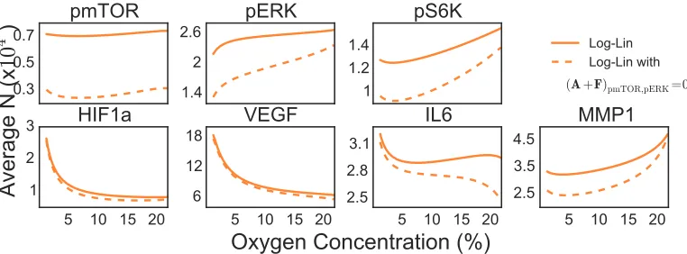
[image:33.612.118.499.74.215.2]

Log-Lin Log-Lin with

Figure 3.7: Predictions from Log-Lin model showing effects of removing removing the effective interaction between pmTOR and pERK.

To test this hypothesis we removed the effective interaction between p-mTOR and p-ERK while keeping the other interactions the same. For simplicity we only show

the effects of this on the average copy number, though this would effect the covari-ance values as well. Changing even one interaction causes significant changes to the

average copy number for some proteins (p-mTOR, p-ERK, p-S6K). This would be

a helpful tool in identifying if more or other drugs were needed to remove multiple interactions to cause the effect of interest, or to be sure to keep some interactions intact (say for some important functions in healthy cells).

Our best fit model also makes useful predictions about the effect of knocking out certain genes to render a protein dysfunctional [26, 27]. In many biological systems

it can be hard to predict the effect of stopping the production or function of a protein in a cell since most protein interactions are not well known and likely vary with cell

0 0.3 0.6

pmTOR

1.4 2

2.6

pERK

0.8 1.1 1.4

pS6K

5 10 15 20 1

2 3

A

ve

ra

ge

N

(x

10

4

)

HIF1a

5 10 15 20 6

12

18

VEGF

5 10 15 20

Oxygen Concentration (%)

2.2 2.6

3.2

IL6

5 10 15 20 2.5

3.5 4.5

hpmTORi=0

[image:34.612.121.500.72.210.2]

MMP1

Log-Lin Log-Lin with

Figure 3.8: Predictions from Log-Lin model showing effects of knocking out pm-TOR.

Here we knockout p-mTOR and as expected p-ERK and p-S6K are largely effected over all oxygen concentration ranges since these are known to be downstream

ef-fectors of p-mTOR. We also see some proteins, IL6 and MMP1, are affected at only one end of the oxygen concentration range which we would not have been able to

predict without this analysis due to the complex interactions of these proteins. This

reinforces the necessity of understanding the evolution of the steady-state distribu-tion, since some effects manifest only under certain perturbation conditions, which would be missed if only one particular steady state was examined.

These predictive capabilities could be extremely useful in understanding how to

effectively drug a protein network in cancer cells. Cancer cells have been shown to be very plastic, so changes in protein networks are frequent and not always lethal.

Similarly, drug sensitivity is dependent on the conditions that the cell is under, as

some cell states are more susceptible to a therapy than others. Describing how many cell states respond to the same perturbation could address this therapeutic challenge.

Specifically, our model can describe both how protein interaction networks evolve,

and which conditions have cell states most susceptible to a drug. Our framework

provides a way that would allow multiple knockouts or interactions to be tested,

C h a p t e r 4

CONCLUSIONS

Summary

We propose a simple theoretical statistical mechanical framework to model the

evo-lution of the probability distribution of cellular components in a cell in response to an external perturbation. We describe a methodology using Bayesian inference,

to extract the functional coupling of a perturbation to the system of interest from

single-cell experimental data. The flexibility of the framework allows the

appli-cation of this methodology to any system where simultaneous measurements of

single-cell cellular component data can be collected. Any number and type of

cel-lular components can be studied, from proteins, to mRNA, to small molecules, such

as metabolites. Even without describing the mechanistic bimolecular interactions,

the results of this approach extract many fundamental underlying characteristics of

the system. It provides a new way to assess and understand the state of the signal-ing network and individual proteins under the influence of a physical or molecular

perturbation.

The application of our framework to explore the effect of hypoxia in GBM cancer cells found that oxygen couples to the effective interactions between proteins, not just to individual proteins. The most probable coupling to the effective interactions was found to be linear, and the individual couplings were found to be either

logarith-mic or linear. These results indicate that the state of the protein interaction network changes linearly with the oxygen concentration, but that this can cause more

com-plex behavior in the fluctuations and average copy number in a cell. We show that

this methodology provides more accurate predictive capabilities than analyses like

the Le Chatelier’s principle method, along with a more detailed description of the

effect of the perturbation.

Future steps

We propose several future experiments that could be done to test the validity of our

approach and also suggest potential systems to investigate.

Further experiments and theoretical analysis can both strengthen and expand the

par-ticularly useful would be 0.1, 10 and 80pO2, could capture a broader range of cell

behaviors by surveying the full spectrum of possible oxygen concentrations. This

additional data could clarify whether the Lin-Lin model is overfitting the current data, or if the Log-Lin model is actually the best fit model. Also to investigate the

observed discontinuity in fluctuations and average copy number, we could change

the way in which we implement our constraints during parameter searches. If the

discontinuity is still observed, then experiments should be done in this low oxygen

concentration regime to check the validity of this unexpected prediction.

Addition-ally, in the raw data there are several outliers (see Fig. 1.1) and some tests with the

removal of these outliers would be a good robustness check.

To determine the need for a more complex model, we propose trying to add a the-oretical ‘extra’ protein for a calculation and remove one of the measured proteins

in another. By removing a protein we could investigate if the most probable

can-didate Hamiltonians order changes leading to a new coupling being predicted. If

a subset of proteins are better described by a different functional form, it may not be appropriate to presume all cell components have the same functional coupling to

the same perturbation. This could indicate that mixed models are perhaps necessary

and should be tested. Adding an ‘extra’ protein would help to identify if the subset

of cellular components experimentally chosen captures enough of the interactions

for this network. For example, it could indicate if some protein had a high influence on this system, we might find that this influence would then be captured in the extra

protein and would help to direct next experiments to include or find this molecule.

Since this theoretical framework is extremely flexible, it can easily be applied to

new systems. In particular, it would be ideal to find a data set for, or experimentally

test, a system that is fully contained (or as much as is possible in biology).

Analo-gous to new methodologies created to examine electronic structures, testing is done

on a well known, well studied and fully understood model systems. Ideally, finding a simple biological system in a cell, consisting of two or three cellular components

and having a well known functional coupling to a perturbation would be ideal.

Per-haps finding a simple two state switching system in which the proteins can be “on”

or “off” may be able to provide this. Additionally, using a more simple model or-ganism as well would be useful, perhapsE.coliwhere there are fewer factors at play and the system is more fully studied.

Once more standardized checks have been completed for the framework, larger

components at a time [2]. It would be interesting to investigate what useful

infor-mation can be provided from understanding how a larger system responds to a

per-turbation. Also, a specific system that this might be useful for, is testing the effects of drug conditions on cancer cells, particularly for finding useful drug

concentra-tions or combinaconcentra-tions by using the convenient predictive tools this methodology

BIBLIOGRAPHY

(1) Vogel, C.; Marcotte, E. M.Nat. Rev. Genet.2012,13, 227–232.

(2) Yu, J.; Zhou, J.; Sutherland, A.; Wei, W.; Shin, Y. S.; Xue, M.; Heath, J. R. Annu. Rev. Anal. Chem.2014,7, 275–95.

(3) Elowitz, M. B.; Levine, A. J.; Siggia, E. D.Science.2002,297, 1183–1186. (4) Maheshri, N.; Shea, E. K. O.Annu. Rev. Biophys. Biomol. Struct.2007, 36,

413–434.

(5) Hart, Y.; Reich-Zeliger, S.; Antebi, Y. E.; Zaretsky, I.; Mayo, A. E.; Alon, U.; Friedman, N.Cell2014,158, 1022–32.

(6) Brock, A.; Chang, H.; Huang, S.Nat. Rev. Genet.2009,10, 336–342. (7) Mettetal, J. T.; Muzzey, D.; Pedraza, J. M.; Ozbudak, E. M.; Oudenaarden,

A. V.Proc. Natl. Acad. Sci.2006,103, 7304–7309.

(8) Hallen, M.; Li, B.; Tanouchi, Y.; Tan, C.; West, M.; You, L. PLoS Comput. Biol.2011,7, 1–16.

(9) Friedman, N.; Cai, L.; Xie, X. S.Phys. Rev. Lett.2006,97, 1–4. (10) Cai, L.; Friedman, N.; Xie, X. S.Nat. Lett.2006,440, 358–362.

(11) Taniguchi, Y.; Choi, P. J.; Li, G.-w.; Chen, H.; Babu, M.; Hearn, J.; Emili, A.; Xie, X. S.Science2011,329, 533–539.

(12) Ocko, S. A.; Mahadevan, L.Phys. Rev. Lett.2015,114, 1–5.

(13) Marchetti, M. C.; Curie, M.; Curie, M. Rev. Mod. Phys. 2013, 85, 1143– 1189.

(14) Toner, J.Phys. Rev. Lett.2012,108, 1–5.

(15) Bertout, J. A.; Patel, S. A.; Simon, M. C.Nat. Rev. Cancer2008,8, 967–975. (16) Brown, J. M.; Wilson, W. R.Nat. Rev. Cancer2004,4, 437–447.

(17) Wouters, B. G.; Koritzinsky, M.Nat. Rev. Cancer2008,8, 851–864. (18) Harris, A. L.; Radcliffe, J.Nat. Rev. Cancer2002,2, 38–47.

(19) Wei, W.; Shi, Q.; Remacle, F.; Qin, L.; Shackelford, D. B.; Shin, Y. S.; Mis-chel, P. S.; Levine, R. D.; Heath, J. R. Proc. Natl. Acad. Sci. U. S. A. 2013, 110, 1352–60.

(20) Foreman-Mackey, D.; Hogg, D. W.; Lang, D.; Goodman, J. Publ. Astron. Soc. Pacific2013,125, 306–312.

(22) Goggans, P. M.; Chi, Y. InAIP Conf. Proc.2004; Vol. 707, pp 59–66. (23) Adler, M.; Mayo, A.; Alon, U.PLoS Comput. Biol.2014,10, 1–14.

(24) Sivia, D.; Skilling, J., Data Analysis: A Bayesian Tutorial, 2nd ed.; OUP Oxford: 2006, pp 79–84.

(25) Cloughesy, T. F. et al.PLos Med.2008,5, 139–151.

(26) Schulze, A.; Downward, J.Nat. Cell Biol. Technol. Rev.2001,3, 190–195. (27) Santiago, Y.; Chan, E.; Liu, P.-q.; Orlando, S.; Zhang, L.; Urnov, F. D.;

A p p e n d i x A

DERIVATIONS USING GRAND CANONICAL ENSEMBLE

This appendix shows the derivations for H = Hofor simplicity. However,

analo-gous derivations can be completed for the full Hamiltonian when a perturbation is

present, since the perturbation terms combined with the reference state terms can simply be thought of as forming ’new’ chemical potentials and effective interactions at each oxygen concentration.

A.1 Partition Function

1-Component System

Assuming cells are at a constant volume and temperature, but particle number

(cel-lular component count) fluctuates, the grand canonical ensemble can be used. The grand canonical partition function is given by

Ξ_o =X

N,E

e−βE+β µN (A.1)

A given microstate in the system is completely determined by the protein copy

number (N) and is weighted according to a Boltzmann distribution. The same

en-ergetics of a given microstate (N) obtained from two different volume and inverse temperature values are given as follows:

βi

Via i

N2+ βiµiN = β

j

Vja j

N2+ βjµjN (A.2)

By setting βi = ξ βj or Vi = ξVj, where ξ is an arbitrary scaling factor, and comparing each term in the above equation shows that the energetics of i and j microstates are equivalent to one another given appropriately rescaled parameters

(aand µ). Therefore volume and beta are redundant and their values are arbitrary.

The partition function can be written as as sum over all discrete particle numbers

since each state will have a different energy according to the particle number:

Ξo=

X

N

e−βH(N) (A.3)

The discrete partition function is not analytically solvable, however, we can

component densities

Ξo =V

Z ∞

0

dρe−βaρ2V+β µρV (A.4)

The exactly solvable Gaussian integral can be evaluated using the following form:

I =

Z ∞

−∞

e−12C x2+Dx_dx (A.5)

where we complete the square as

−1

2C x

2₊

Dx =−1

2C(x− D C)

2₊ D2

2C (A.6)

WhenC =2a, D= µandx = ρ, the partition can be solved as

Ξ_o =V

Z ∞

0

dρeβV(−a(ρ−2µa)2+

µ2

4a) _(A.7)

Ξ_o =V eβVµ

2 4a

Z ∞

0

dρe−βV aρ2 (A.8)

Ξ_o= V

2

r π

βV ae

βVµ2

4a _(A.9)

n-Component System

With n cellular components, the partition function can be written by integrating over the density for each component.

Ξ_o =Vn

Z ∞

0

dρ1

Z ∞

0

dρ2. . .

Z ∞

0

dρneβV(− P

i,i<jai jρiρj+Piµiρi) _(A.10)

As with the 1-component case, this exponential can be rewritten to complete the

square with the use of matrix form as

Ξ_o =Vn

Z ∞

0

dρ1

Z ∞

0

dρ2. . .

Z ∞

0

dρne−

1

2ρTAρ+MTρ _(A.11)

whereρ=

* . . . . . . . , ρ1 ρ2 ... ρn + / / / / / / /

-,MT= βV µ1 µ2 . . . µn

andA=2βV

* . . . . . . . ,

a11 1₂a12 . . . 1₂a1n

1

2a21 a22 . . . 1

2a2n

... ... ... ...

1

2an1

1

2an2 . . . ann + / / / / / / /

This equation can be simplified by transforming ρ to another vector q with an

orthogonal matrixSwith a determinant of unity:

ρ=Sq (A.12)

The integral is now

Ξ_o=Vn

Z ∞

0

dq1

Z ∞

0

dq2. . .

Z ∞

0

dqne−

1 2qTS

−1_ASq+MT_Sq

(A.13)

The matrixSis a diagonalizing matrix which means that

S−1AS=*. . .

,

d1 0 . . .

0 d2 . . .

... ... ... + / / /

-= D (A.14)

which transforms as

−1

2ρ

T_Aρ+MT_{ρ→ −}1

2q

T_Dq+MT_{Sq (A.15)}

The variables can now be separated, which expands to

−1

2(d1q

2

1+d2q22+. . .dnqn2)+ MαSα1q1+ MαSα2q2+. . .MαSαnqn (A.16)

where the summation of terms will be over the index α. The square can be com-pleted for eachqi term.

−1

2di(qi−

MαSαi

di

)2+ (MαSαi)

2

2di

(A.17)

Using the completed square the partition function can be evaluated as

Ξo= (

V 2)

n(2π)

n

2

|A|12

e12MTA

−1_M

(A.18)

where|A|is the determinant of a A.

A.2 HoEnsemble Statistics

The average,hNi, and fluctuations,h(δN)2i, in cellular component copy number are calculated from the derivative of the partition function with respect to its conjugate

variable β µaccording to the following equations:

hNi= 1

β ∂lnΞ