On source coding for networks

(1)

On Source Coding for Networks

Thesis by Michael Fleming

In Partial Fulfillment of the Requirements for the Degree of

Doctor of Philosophy

California Institute of Technology Pasadena, California

2004

(2)

c

2004

(3)

iii

(4)

Acknowledgments

I would like to express my immense gratitude to my advisor, Professor Michelle Effros, whose guidance and mentoring made this work possible.

I would like to thank the members of my candidacy and defense committees, Professors Jehoshua Bruck, Michelle Effros, Gary Lorden, Babak Hassibi, Steven Low, and Robert McEliece, who read my thesis manuscript and gave me valuable feedback on my work.

My labmates Diego Dugatkin, Hanying Feng, Qian Zhao, Wei-Hsin Gu, and especially Sidharth Jaggi, helped me with technical details and provided much-appreciated company during long writing sessions. I am grateful also to Jason Colwell and Professor Sze Tan for their advice on optimization and estimation theory.

I would like to thank my family and friends for their constant support throughout my time at Caltech.

Finally, I am grateful to the agencies that funded my research. This work was supported by the F.W.W. Rhodes Memorial Scholarship and a Redshaw Award, the William H. Pick-ering Fellowship, NSF Grant Nos. MIP-9501977, CCR-9909026, and CCR-0220039, the Lee Center for Advanced Networking at Caltech, the Intel Technology for Education 2000 pro-gram, and a grant from the Charles Lee Powell Foundation.

(5)

(6)

Abstract

In this thesis, I examine both applied and theoretical issues in network source coding.

The applied results focus on the construction of locally rate-distortion-optimal vector quantizers for networks. I extend an existing vector quantizer design algorithm for arbitrary network topologies [1] to allow for the use of side information at the decoder and for the presence of channel errors. I show how to implement the algorithm and use it to design codes for several different systems. The implementation treats both fixed-rate and variable-rate quantizer design and includes a discussion of convergence and complexity. Experimental results for several different systems demonstrate in practice some of the potential performance benefits (in terms of rate, distortion, and functionality) of incorporating a network’s topology into the design of its data compression system.

The theoretical work covers several topics. Firstly, for a system with some side informa-tion known at both the encoder and the decoder, and some known only at the decoder, I derive the rate-distortion function and evaluate it for binary symmetric and Gaussian sources. I then apply the results for binary sources in evaluating the binary symmetric rate-distortion function for a system where the presence of side information at the decoder is unreliable. Previously, only upper and lower bounds were known for that problem. Secondly, I address

(7)

(8)

List of Figures

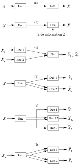
1.1 (a) A point-to-point network. (b) A side information network. (c) A two-user MA network. (d) A two-receiver MR network. (e) A two-channel MD network. (f) A two-receiver BC network. . . 5 1.2 The relationship between the systems. . . 6 1.3 (a) The mixed side information system considered in Chapter 4. (b) The

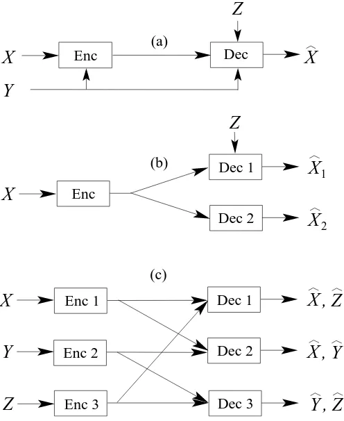
system of Heegard and Berger [2] and Kaspi [3]. (c) The encoder, three-decoder system considered in Chapter 5. . . 8

2.1 (a) The conditional rate-distortion network [4]. (b) The network of Berger and Yeung [5]. (c) The network of Kaspi and Berger [6]. . . 14

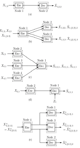
3.1 (a) A point-to-point code. (b) A two-receiver BC code. (c) A two-user MA code. (d) A WZ code with side informationZ1. (e) A two-channel MD code. The notation is Xt,S for a source and ˆXt,S,r for a reproduction; here t is the transmitter,S the set of receivers, and r the reproducer. . . 32 3.2 A general three-node network. . . 33 3.3 The 2AWZ network. . . 44

(11)

LIST OF FIGURES xi 3.4 A discrete Markov constraint example. (a) The distribution P, uniform over

an ellipse. (b,c,d) ˆP for _|K2,1| = |K3,1| = K when: (b) K = 21, (c) K = 23, (d) K = 25_{. . . .} ₅₂

3.5 Optimal encoding at node 2. (a) The estimated performance for a given index set i2,∗ can be found by summing the performance in two linked 2AWZ

subsystems. (b),(c) The two subsystems. . . 56

3.6 (a) WZVQ performance as a function of side information rate log2(|KZ|)/nfor jointly Gaussian source and side information (ρ= 0.375). (b) Various coding performances for the 2AWZ system on satellite data. . . 59

3.7 (a) Comparison of fixed- and variable-rate coding performances for the 2A system. (b) WZ code performance as a function of source and side information correlation and the number of cosets used in decoder initialization. . . 61

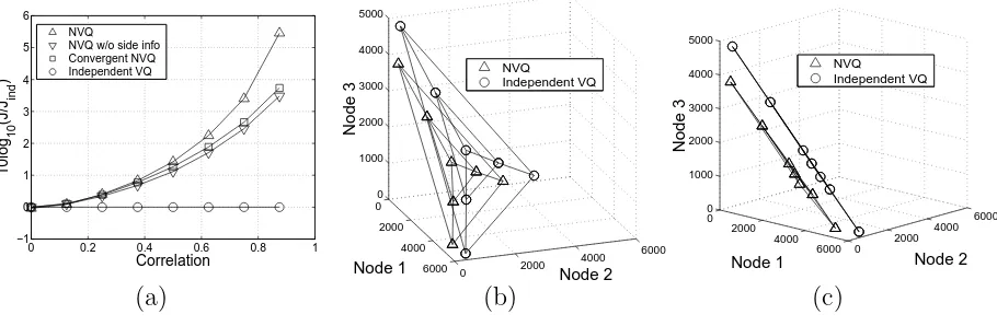
3.8 Efficiency of network source coding vs. independent coding. (a) Overall per-formance as a function of correlation. (b),(c) Weighted sum distortion at each node as a function of the Lagrangian parameters (shown from two different angles). . . 63

(12)

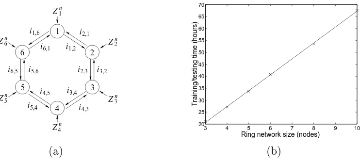
3.10 (a) The network messages and side informations of a six-node ring network.

(b) Design time for a ring network. . . 67

4.1 (a) The conditional rate-distortion system. (b) The Wyner-Ziv system. (c) The MSI system. (d) Heegard and Berger’s system. . . 73

4.2 A distribution achieving RX|Y Z(p, D). Here a= 1−Dl11 and N is Gaussian noise, independent of (X, Y, Z), with mean zero and variance D/(1₋Dl11). . 82

4.3 Joint distribution of (X, Y, Z) for binary MSI example. . . 82

4.4 Joint distribution of (W, X, Z) for_{|W| ≤}3. . . 83

4.5 The value (top) and the form (bottom) of the optimal solution for different values of p0 and q0 when D= 0.1. . . 89

4.6 Numerical results for Heegard and Berger’s system,q0 = 0.1, D1 = 0.05. . . . 94

5.1 A bipartite graph considered for the feedback problem. . . 96

5.2 The lossless coding system used in the proof of Theorem 18. . . 99

5.3 A general network. The line is an example of a cutset boundary separating the M nodes of the network into two sets, A and B. . . 103

5.4 The simplified network for the cutset bounds. . . 105

5.5 The system used for the three-set extension of the cutset approach. . . 106

5.6 (a) A two-user MA network. (b) A three-node network. . . 108

5.7 A k-ary broadcast tree. . . 110

5.8 A broadcast system with three receivers. . . 118

(13)

LIST OF FIGURES xiii A.1 Sample images from the GOES-8 weather satellite. From left to right: visible

spectrum, infrared 2, infrared 5. . . 131

(14)

List of Tables

1.1 Progress chart for network source coding. . . 6

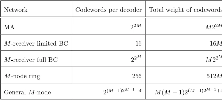
3.1 Application of the Markov constraint to a pair of Gaussian sources. . . 51 3.2 Total number of codewords for various systems. . . 68

4.1 Possible decoding functions for each symbol, together with their expected distortion contribution. . . 85 4.2 A possible decoding function f when _|W|= 3. . . 85

A.1 Data source assignments for the NVQ experiments . . . 131

(15)

Chapter 1 Introduction

The amount of data transferred over electronic communication networks has increased dra-matically in the last three decades. As a result, the motivation for developing efficient source codes for network data compression has never been higher. Yet, despite the growing number of network applications, there are very few source codes in common use that take advantage of the topology of the network in which they operate. Indeed, the vast majority of data compression codes are developed without any consideration whatsoever of the structure of the network; the network is treated as a collection of independent point-to-point links, and a separate code is designed for each link. This “independent” approach to source code design for networks does not achieve the goal of using the network links in the most efficient man-ner. Although point-to-point codes remove the redundancy in each individual source, they are unable to remove the redundancy between different sources, and are therefore inefficient when applied to statistically dependent sources.

Redundancy between data sources is observed in a growing number of network applica-tions. Video conferencing, sensor networks, and distributed computing all generate multiple,

(16)

highly correlated data streams. These applications require a global, “network” approach to code design, one that exploits inter-source dependencies. This observation begs the question of why such an approach is rarely taken in practice. One reason is an incomplete understand-ing of the magnitude of the potential benefits; rate-distortion results are known for only a few simple networks. Another, perhaps more important reason is a lack of understanding of how to convert existing theory into good practical codes. Indeed, even the definition of “goodness” in networks is not immediately clear. Several factors must be balanced: rates, distortions, design complexity, run-time encoding and decoding complexity, and robustness to changes or failures in the network.

(17)

3 both fixed- and variable-rate quantizer design and take into account the presence of channel errors. However, the implementation of variable-rate design is currently limited due to the lack of lossless entropy codes for general networks. The range of systems for which optimal variable-rate quantizers can be designed will expand as the field of lossless network source coding develops. I design VQs for several different systems and evaluate their performance compared to both an independent coding approach and to rate-distortion bounds. The ex-perimental results demonstrate that, for networks with correlated sources, incorporating the network’s topology into the design of its data compression system yields significant increases in performance with respect to an independent coding approach. This work also appears in [7, 8, 9].

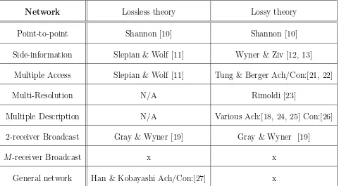
Development of more efficient practical codes is supported by a more thorough under-standing of source coding theory, which is the focus of the second part of this thesis. Table 1.1 summarizes our current knowledge of source coding theory for the basic network classes il-lustrated in Figure 1.1. In this table, a citation in one of the table cells indicates that we know the region of achievable rates (for lossless coding) or the rate-distortion function (for lossy coding). Partial knowledge of the rate-distortion function via an achievability (ach) or converse (con) result is as indicated. An ‘x’ denotes that the area remains largely open. The various systems mentioned are introduced briefly below.

• Point-to-point [10]: A point-to-point network, shown in Figure 1.1(a), is the simplest communication network. A single encoder transmits information to a single decoder.

• Side information1 _{(SI) [11, 12, 13]:} _{A SI network, shown in Figure 1.1(b), is a}

1

(18)

point-to-point communication network in which side information is available at the decoder. In the context of lossy coding, I refer to this system also as the Wyner-Ziv (WZ) system.

• Multiple Access (MA) [11]: In an MA network, shown in Figure 1.1(c), two or more senders transmit information to a single receiver.

• Multi-Resolution (MR) [14, 15]: MR codes, shown in Figure 1.1(d) generate an embedded source description for two or more receivers. Receiver i receives only the first fraction fi of the description, where f1 < f2 < . . ..

• Multiple Description (MD) [16, 17, 18]: An MD code can be used for point-to-point communication over multiple, unreliable communication channels (or over a lossy, packet-based channel in which lost packets cannot be retransmitted). Each channel’s source description may be lost, and the decoder reproduces the source by combining all received descriptions. In Figure 1.1(e), we model a two-channel system and represent the different decoding scenarios with three separate decoders.

• Broadcast (BC) [19, 20]: In a BC network, shown in Figure 1.1(f), a single sender describes a collection of sources to two or more receivers. A different message can be transmitted to each possible subset of the receivers.

The relationships between the various systems are shown in Figure 1.2. Point-to-point net-works are special cases of both MA and BC netnet-works. SI netnet-works are considered as special

available only at the decoder. When side information is available to both encoder and decoder, I use the

(19)

5

X

,

X

,

X

[image:19.612.197.463.68.623.2]

(b) Dec 2 (d) (a) (c)

X

Enc Enc Dec Dec Enc 1 Enc 2 Dec Dec 1 Enc Dec 12 Dec 2 Enc Dec 1 Dec 1 Dec 2 Enc

Z

(e) (f) 2 1 1 2 1 2 1 2 12 2 1 2 1 Side information

(20)

General Networks MA BC

Point−to−point

General Networks BC

MR

Point−to−point MD

General Networks

Point−to−point

[image:20.612.91.572.339.604.2]

MA SI

Figure 1.2: The relationship between the systems.

Network Lossless theory Lossy theory

Point-to-point Shannon [10] Shannon [10]

Side-information Slepian & Wolf [11] Wyner & Ziv [12, 13] Multiple Access Slepian & Wolf [11] Tung & Berger Ach/Con:[21, 22]

Multi-Resolution N/A Rimoldi [23]

Multiple Description N/A Various Ach:[18, 24, 25] Con:[26] 2-receiver Broadcast Gray & Wyner [19] Gray & Wyner [19]

M-receiver Broadcast x x

General network Han & Kobayashi Ach/Con:[27] x

(21)

7 cases of MA networks for which one source (the side information) has no rate constraint. MR and MD networks are both special cases of the M-receiver BC network.

Consider now the specific example of an environmental remote sensing network with sev-eral sensors, each of which takes measurements and transmits them to a central base station, which also makes its own measurements. In encoding its transmission to the base station, each sensor can consider the measurements taken by the base station as side information available to the base station’s decoder. If the system uses multi-hop transmissions, then measurements relayed by a sensor act as side information available both to that sensor’s encoder and the base station’s decoder. Motivated by this framework, I begin the second part of the thesis in Chapter 4 by deriving rate-distortion results for two systems using side information. First, for the system shown in Figure 1.3(a) with some side information known at both the encoder and the decoder, and some known only at the decoder, I derive the rate-distortion function and evaluate it for binary symmetric and Gaussian sources. I then apply the results for the binary source to a second network, shown in Figure 1.3(b), which models point-to-point communication when the presence of side information at the decoder is unreliable [2, 3]. I demonstrate how to evaluate the binary rate-distortion function for that network, closing the gap between previous bounds [2, 28] on its value. The form of the binary rate-distortion function for this second system exhibits an interesting behavior akin to successive refinement, but with side information available to the refining decoder. This work also appears in [29, 30]

(22)

(a)

(b)

Enc Dec

Z

Enc

Dec 1

Dec 2

X

Y

X

(c) Enc 1

Enc 2

Enc 3

Dec 2 Dec 1

Dec 3

X

Z

,

X

Z

,

Y

,

X

Y

Z

[image:22.612.200.448.192.495.2]

2 1

(23)

9 when an encoder does not have access to all of the messages or side informations available to the decoder. However, the Slepian-Wolf result [11] implies that this result does not carry over to the lossless case. This begs the question of whether feedback from a decoder to an encoder can ever reduce the rate total rate required in lossless coding. I answer this question by means of a detailed example which shows that, as the alphabet size of the sources grows without bound, feedback of a limited rate can reduce by an arbitrary amount the total rate required by the encoders. The second topic is the development of simple rate-distortion converses for networks. Network converses are often difficult to find, but I show that a method based on cutsets yields simple converses for any lossy source coding network. This approach has the advantage of easy applicability but the drawback that the converses are, in many cases, fairly loose. Finally, motivated by the lack of results in general broadcast coding, I look at the rate tradeoff between the three encoders in the three-source three-receiver lossless network of Figure 1.3(c) and apply the outcome to the derivation of an achievability result for three-receiver lossy broadcast source coding. I also derive a rate-distortion result for a tree-structured broadcast coding system.

(24)

Chapter 2 Background

This chapter defines typical sequences, summarizes several existing results in network rate-distortion theory, and summarizes past work in VQ coding. For the rate-rate-distortion results, I present the definition of the achievable rate-distortion region in detail only for the point-to-point network; a similar definition applies for each of the other networks.

2.1 Jointly Typical Sequences

The rate-distortion proofs in this thesis make use of strongly jointly typical sequences as defined below.

Let {Xk}K_k=1, with Xk ∈ Xk ∀k, denote a finite collection of discrete random variables with some fixed joint distribution p(x1, x2, . . . , xK). Let S denote an ordered subset of the indices _{1,2, . . . , K_} and letXS = (Xk :k ∈S). Denoten independent samples of XS ∈ XS by Xn

S = (XS,1, . . . , XS,n). For any S and any a(S)∈ X(S), let

N(aS|xnS) = n

X

i=1

1xS,i=aS,

(25)

2.2. EXISTING RATE-DISTORTION RESULTS 11 where xS,i is the ith element ofxnS and 1E is the indicator function for event E.

Definition The set A∗(n) of -strongly typical n-sequences is the set of all sequences (xn

1, xn2, . . . , xnK) satisfying for allS ⊆ {X1, X2, . . . , XK} the following two conditions: 1. For all aS ∈ XS with p(aS)>0,

1

nN(aS|x

n

S)−p(aS)

<

|XS|

.

2. For all aS ∈ XS with p(aS) = 0, N(aS|xnS) = 0.

The following two lemmas describe useful properties of the strongly typical set.

Lemma 1 [31, Lemma 13.6.1] Let XS,1, . . . , XS,n be drawn i.i.d. with distribution p(xS).

Then

Pr(A∗(n))_→1 as n _{→ ∞}.

Lemma 2 [31, Lemma 13.6.2] Let Y1, . . . , Yn be drawn i.i.d. with distribution p(y). For

xn

∈A∗(n), the probability that (xn, Yn)∈A∗(n) is bounded by

2−n(I(X;Y)+1) _≤ _Pr((_xn_{, Y}n₎_∈_A∗(n)

)≤2

−n(I(X;Y)−1)_,

where 1 →0 as →0 and n→ ∞.

2.2 Existing Rate-Distortion Results

2.2.1 The Point-to-Point Network

(26)

and let d : _{X ×}_{X →}ˆ [0,_∞) be a measure of the distortion between symbols from the two alphabets.

A (2nR_{, n,}_{∆n) point-to-point rate-distortion code for source} _X _{under distortion measure}

d is defined by encoder and decoder functions (αn_{, β}n_{) such that}

αn _:

Xn

→ {1,2, . . . ,2nR

}

βn _:

{1,2, . . . ,2nR

} →Xˆn ∆n = 1

n

X

i=1

Ed(Xi,Xˆi),

where ˆXi is the ith component of ˆXn =βn(αn(Xn)) and the expectation is with respect to the source distribution. A rate-distortion pair (R, D) is achievable if there exists a sequence of (2nR_{, n,}_{∆n) rate-distortion codes (}_αn_{, β}n_{) with limn}

→∞∆n ≤ D. The rate-distortion

region is defined as

R=_{(R, D) : (R, D) is achievable_},

where the overbar denotes set closure. The rate-distortion function is defined as

RX(D) = inf

D {R : (R, D)∈ R}.

The following theorem gives an information-theoretic characterization of the rate-distortion function.

Theorem 1 [10, Section 28]

RX(D) = inf ˆ

X∈MX(D)

I(X; ˆX),

where MX(D)is the closure of the set of all random variables Xˆ described by a test channel

(27)

2.2. EXISTING RATE-DISTORTION RESULTS 13 The infimum above has been evaluated for a variety of sources, including binary and Gaussian sources (see, for example, [31]). For i.i.d. sources, it can be evaluated numerically via a globally-optimal iterative descent algorithm [32, 33].

2.2.2 The Conditional Rate-Distortion Network

When side information Y ∈ Y is available to both encoder and decoder, as in Figure 2.1(a), the rate-distortion function is called the conditional rate-distortion function and is given by the following theorem.

Theorem 2 [4, Pg. 8]

RX|Y(D) = inf ˆ

X∈MX|Y(D)

I(X; ˆX_|Y),

where MX|Y(D)is the closure of the set of all random variablesXˆ described by a test channel

p(ˆx|x, y) such that Ed(X,Xˆ)≤D.

The infimum above has been evaluated for jointly Gaussian sources [13].

2.2.3 The Wyner-Ziv Network

When side information Z ∈ Z is available to only the decoder and not to the encoder, as in Figure 1.1(b), the rate-distortion function is called the Wyner-Ziv (WZ) rate-distortion function. The following theorem gives its form for both discrete and continuous sources, but for continuous sources the achievability part of the theorem is proven only for distortion measures satisfying the following two conditions:

(28)

[image:28.612.189.458.67.325.2]

X

(a)

X

Enc Dec

X

Y

(b)

,

Dec Enc 1 Enc 2

X

(c)

,

Enc 1 Enc 2 Dec 1 Dec 2

X

1 2 1 2,2 2,1 1 2 2 1

Figure 2.1: (a) The conditional rate-distortion network [4]. (b) The network of Berger and Yeung [5]. (c) The network of Kaspi and Berger [6].

2. For all random variables ˆX such that 0 < Ed(X,Xˆ) < _∞ and all > 0, there exists a finite subset _{xˆ1, . . . ,xˆN} ⊆ Xˆ, and a quantizer fQ : ˆX → {Xˆi} such that

Ed(X, fQ( ˆX))≤(1 +)Ed(X,Xˆ).

Condition 2 is a smoothness constraint used in generalizing the WZ rate-distortion proof from discrete to continuous alphabets [13]. Wyner notes that it is not especially restrictive, showing that when _X = ˆ_X = IR it holds for all r-th power distortion measures, d(x,xˆ) =

|x−xˆ|r _with _{r >}_0.

Theorem 3 [12, Theorem 1], [13, Theorems 2.1,2.2]

RX|{Z}(D) = inf

W∈MX|{Z}(D)

I(X;W|Z)

= min

W∈MX|{Z}(D)

(29)

2.2. EXISTING RATE-DISTORTION RESULTS 15

where _MX|{Z}(D) is the closure of the set of all random variables W such that W →

X _→ Z forms a Markov chain and there exists a function f : _{W × Z →} _Xˆ for which

Ed(X, f(W, Z))≤D.

The set notation around theZ in the descriptor RX|{Z}(D) denotes that the side information

is available only at the decoder. Roughly speaking, the Markov chain condition in the state-ment of Theorem 3 reflects the restriction that the description chosen by the encoder must be based onX alone since the encoder does not have direct access toZ. The WZ rate-distortion function has been evaluated for both binary symmetric [12] and jointly Gaussian [13] sources.

2.2.4 The Multiple-Access Network

In the two-user MA network of Figure 1.1(c), dependent sources X1 and X2 are described by two separate encoders to a single decoder. Encoder 1 uses rate R1 and encoder 2 uses rate R2. The decoder makes reproductions ˆX1 and ˆX2 satisfying the distortion constraints

Ed(Xi,Xˆi)≤Di, i= 1,2.

Let _RM A(D1, D2) be the closure of the set of all achievable rate vectors for distortions (D1, D2). A complete single-letter characterization of RM A(D1, D2) is not available, but achievability and converse results exist. Berger and Tung [34, 21, 22] give the following results. Define _Rach(D1, D2) to be the closure of the set of all rate pairs (R1, R2) for which there exist auxiliary random variables W1 and W2 such that

1.

R1 ≥ I(X1, X2;W1|W2)

R2 ≥ I(X1, X2;W2|W1)

(30)

2. There exist functions f1(W1, W2) and f2(W1, W2) satisfying

Ed(Xi, fi(W1, W2)) ≤ Di, i= 1,2.

3. W1 →X1 →X2 →W2 forms a Markov chain.

Define Rcon(D1, D2) similarly, but replace the Markov requirement in condition 1 with the requirements thatW1 →X1 →X2 and X1 →X2 →W2 form Markov chains.

Theorem 4 [21, Theorem 4.1,5.1], [22, Theorem 6.1,6.2]

Rach(D1, D2)⊆ RM A(D1, D2)⊆ Rcon(D1, D2)

Berger and Tung provide theM-user extension of the above and evaluate the two-user region for joint Gaussian sources in [34, 21]. Oohama derives further results for joint Gaussian sources in [35, 36].

Berger and Yeung give a matching achievability and converse for the case D1 = 0 in [37]. In that case, let R∗₍_D_{2) be the closure of the set of all rate pairs (}_R

1, R2) for which there exists an auxiliary random variables W2 such that

1.

R1 ≥ H(X1|W2)

R2 ≥ I(X2;W2|X)

R1+R2 ≥ H(X) +I(X2;W2|X).

2. A function f2(X, W2) exists satisfying Ed(X2, f2(X, W2))≤D2. 3. X1 →X2 →W2 forms a Markov chain.

(31)

2.2. EXISTING RATE-DISTORTION RESULTS 17 Theorem 5 [37, Theorem 1]

RM A(0, D2) =R∗₍_D₂₎

The above region is determined almost completely for jointly symmetric binary sources [37]. Kaspi and Berger [6] look at how inter-encoder communication affects the rate-distortion region by adding a common link of rate R0 from encoder 1 to encoder 2 and the decoder, as shown in Figure 2.1(b). Their result is the following. Let_RKB(D1, D2) be the closure of the set of all achievable rate triples for distortions (D1, D2). Let Rach be the closure of the set of all rate triples for which there exist auxiliary random variables U1, U2, and W such that 1.

R0 ≥ I(X2;W|X1)

R1 ≥ I(X1;U1|U2, W)

R2 ≥ I(X2;U2|U1, W)

R0+R1+R2 ≥ I(X1, X2;U1, U2, W).

2. There exist functions f1(U1, U2, W) andf2(U1, U2, W) satisfying Ed(Xi, fi(U1, U2, W))≤

Di, i= 1,2.

3. U1 →(X1, W)→(X2, W)→U2 and X1 →X2 →W form Markov chains. 4. |U| ≤ |X1||X2|+ 6|X1|+ 5, |U2| ≤ |X2|2+ 6|X2|+ 5, |W| ≤ |X2|+ 6.

Theorem 6 [6, Theorems 2.1 - 2.5]

Rach(D1, D2)⊆ RKB(D1, D2),

with equality in the following (not necessarily exhaustive) cases:

(32)

2.2.5 Multiple Access with Encoder Breakdown

Consider the case whenD1 = 0, but there exists a chance that the encoder forX1 may break down. This can be modeled by the system of Figure 2.1(c) using two decoders. Decoder 1 corresponds to the case when the encoder of X1 does not break down; decoder corresponds to the case when it does. Here X1 is described at rate R1 to decoder 1 and X2 is described at common rate R2 to both decoders. X1 must be reproduced losslessly at decoder 1 and

X2 must be reproduced to distortion D21 at decoder 1 and distortion D22 at decoder 2. Berger and Yeung [5] give the following characterization of the rate-distortion region. Let

RM AEB(D21, D22) be the closure of the set of all achievable rate vectors for distortions (D21, D22). Let R∗(D21, D22) be the closure of the set of all rate pairs (R1, R2) for which there exist auxiliary random variables U and V such that

1.

R1 ≥ H(X1|U)

R2 ≥ I(X2;U) +I(X2;V|X1, U).

2. There exist functions ˆX21=f1(X1, U, V) and ˆX22 =f2(U) satisfying

Ed(X2, f1(X, U, V)) ≤ D21

Ed(X2, f2(U)) ≤ D22.

3. X1 →X2 →(U, V) forms a Markov chain. 4. |U| ≤ |X2|+ 3, |V| ≤ |X2|+ 3.

Theorem 7 [5, Theorem 1]

RM AEB(D21, D22) =R∗(D21, D22)

(33)

2.2.6 The Multi-Resolution Network

Figure 1.1(d) shows two-receiver MR coding. A single sourceX is described to two decoders. Both decoders receive a common description at rateR1, and decoder 2 receives an additional private description at rateR2. Decoders 1 and 2 make reproductions ˆX1and ˆX2 at distortions

D1 and D2 ≤ D1, respectively. The rate-distortion region is given by Rimoldi [23]. Let

RM R(D1, D2) be the closure of the set of all achievable rate vectors for distortions (D1, D2), and letR∗₍_D

1, D2) be the closure of the set of all rates for which there exist ˆX1 and ˆX2 such that

R1 ≥ I(X; ˆX1)

R2 ≥ I(X; ˆX2|Xˆ1)

Ed(X,Xˆ1) ≤ D1

Ed(X,Xˆ2) ≤ D2.

RM R(D1, D2) =R∗(D1, D2).

An M-receiver result is also given in [23]. The rate distortion region has been evaluated for several sources; for more details see the discussion on successive refinement in Section 2.2.10.

2.2.7 The Multiple Description Network

(34)

makes reproduction ˆX2; decoder 12 receives both descriptions and makes reproduction ˆX12. Let _RM D(D1, D2, D12) be the closure of the set of all achievable rate vectors for distor-tions (D1, D2, D12). An exact single letter characterization of RM D(D1, D2, D12) remains unknown, but achievability and converse results exist. El Gamal and Cover [18] give the following achievability result. Let _Rach(D1, D2, D12) be the closure of the set of all rates (R1, R2) for which there exist ˆX1, ˆX2, and ˆX12 such that

R1 ≥ I(X; ˆX1)

R2 ≥ I(X; ˆX2)

R1+R2 ≥ I(X; ˆX12,Xˆ1,Xˆ2) +I( ˆX1; ˆX2)

Ed(X,Xˆt) _≤ Dt, t ∈ {1,2,12}.

Rach(D1, D2, D12)⊆ RM D(D1, D2, D12).

Ahlswede shows that this achievability result is tight for the special case of multiple descrip-tion coding in which R1+R2 =RX(D12) [38], and Ozarow shows that it is tight for Gaussian sources [17]. However, Zhang and Berger show it to be loose in general [24]. They provide both a counterexample to its tightness and the following new achievable region. Redefine

Rach(D1, D2, D12) to be the closure of the set of all rates (R1, R2) for which there exist aux-iliary random variables ˆX0, ˆX1, ˆX2 such that

1.

Ri ≥ I(X; ˆX0,Xˆi), i= 1,2

(35)

2.2. EXISTING RATE-DISTORTION RESULTS 21 2. There exist functions fi( ˆX0,Xˆi),i= 1,2, and f12( ˆX0,Xˆ1,Xˆ2) satisfying

Ed(X, fi( ˆX0,Xˆi)) ≤ Di, i= 1,2

Ed(X, f12( ˆX0,Xˆ1,Xˆ2)) ≤ D12.

Rach(D1, D2, D12)⊆ RM D(D1, D2, D12),

A generalization of this result to M descriptions is given in [25].

The following converse for MD is provided by Sher and Feder [26]. Let _Rc(D1, D2, D12) be the closure of the set of all rates (R1, R2) for which there exist ˆX1, ˆX2, and ˆX12such that

R1 ≥ I(X; ˆX1)

R2 ≥ I(X; ˆX2)

R1+R2 ≥ I(X; ˆX12|Xˆ1,Xˆ2) +I(X; ˆX1) +I(X; ˆX2)

Ed(X,Xˆt) ≤ Dt, t∈ {1,2,12}.

RM D(D1, D2, D12)⊆ Rc(D1, D2, D12).

2.2.8 The Network with Unreliable Side Information

(36)

Kaspi [3]. They give different but equivalent characterizations of the rate-distortion region; I state here Heegard and Berger’s result. Let _RU SI(D1, D2) be the closure of the set of all achievable rate vectors for distortions (D1, D2), and letR∗(D1, D2) be the closure of the set of all rates R for which there exist auxiliary random variablesU and V such that

1.

R ≥ I(X;U) +I(X;V|U, Z).

2. There exist functions f1(U, V, Z) and f2(U) satisfying

Ed(X, f1(U, V, Z)) _≤ D1

Ed(X, f2(U)) _≤ D2.

3. X _→Z _→(U, V) forms a Markov chain. 4. |U| ≤ |X |+ 2 and |V| ≤(|X |+ 1)2_.

RU SI(D1, D2) =R∗(D1, D2)

(37)

2.2.9 The Two-Receiver Broadcast Network

Figure 1.1(f) shows a two-receiver BC network. Source X1 must be described to decoder 1, and sourceX2 must be described to decoder 2. There are three channels for the descriptions; a common channel to both decoders of rate R12, and two private channels, one to each of the two decoders, of rates R1 and R2, respectively. The rate-distortion region is given by Gray and Wyner [19]. Let _RBC(D1, D2) be the closure of the set of all achievable rate vectors for distortions (D1, D2), and let R∗(D1, D2) be the closure of the set of all rate pairs (R1, R2) for which an auxiliary random variable W exists satisfying

R12 ≥ I(X1, X2;W)

R1 ≥ RX1|W(D1)

R2 ≥ RX2|W(D2).

RBC(D1, D2) =R∗(D1, D2)

I generalize the achievability result to the three receiver case in Chapter 5. I also derive tight results for a special case of M-receiver broadcast coding.

2.2.10 Rate Loss and Successive Refinement

Zamir [39] defines the rate loss L(D) for WZ coding as the difference between the WZ and the conditional rate-distortion functions; thus L(D) = RX|{Z}(D)−RX|Z(D). The rate loss

(38)

decoder compared to when it is available to both the encoder and the decoder. It is always non-negative.

In [39], Zamir shows that for a continuous source and the r-th power distortion measure, the rate loss is bounded by a constant which depends on the source alphabet and the dis-tortion measure, but not on the source distribution. For example, for continuous alphabet sources and squared-error distortion,L(D)≤ 1

2 for allD. This bound shows that the penalty paid for Y not being available at the encoder cannot be arbitrarily large.

The concept of rate loss can be applied to other coding scenarios such as MR coding [40]. For MR codes, rate loss is found to be zero for successively refinable sources, defined below. Definition[14] [15, Definitions 1 and 2] A sourceX is said to besuccessively refinableunder a distortion measure if, for that source and distortion measure, successive refinement from distortion D1 to distortion D2 is achievable for every D1 ≥D2. Successive refinementfrom distortion D1 to D2 ≤D1 is said to be achievable if there exists a sequence of encoding and decoding functions

αn₁ : Xn

→ {1, . . . ,2nR1_}

αn1 : Xn→ {1, . . . ,2n(R2−R1)}

βn

1 : {1, . . . ,2nR1} →Xˆn

βn

2 : {1, . . . ,2nR1} × {1, . . . ,2n(R2−R1)} →Xˆn

such that for ˆXn

1 =β1n(α1n(Xn)) and ˆX2n =β2n(αn1(Xn), αn2(Xn)),

lim sup n→∞

Ed(Xn_,_X_ˆn

1) ≤ DX(R1) lim sup

n→∞ Ed(X

n_,_X_ˆn

(39)

2.3. VECTOR QUANTIZATION 25 where DX(R) is the distortion-rate function for the source.

Examples of successively refinable sources include Gaussian sources under squared-error distortion, arbitrary discrete distributions under Hamming distortion, and Laplacian sources under absolute error [15]. An example of a problem that is not successively refinable is that of the Gerrish source [41, 15] (which has _{|X |} = 3 and p(x) = (1−₂p, p,1−₂p)), although the maximal excess rate R2−RX(D2) when R1 =RX(D1) is very small [42].

Rate loss results for MR codes [40, 43] bound the difference in total rate Pk

i=1Ri used to achieve distortionDiin resolutioniand the corresponding rateRX(Di) for an optimal point-to-point code. They give source-independent bounds similar to those of Zamir for the WZ system and show that only a small penalty is paid in using a single multi-resolution source description in place of a family of optimal point-to-point (single-resolution) descriptions.

2.3 Vector Quantization

Past work on VQ design typically takes one of two approaches. Either the codebook is first initialized in some way and then trained using an iterative descent algorithm (“uncon-strained” design), or a lattice or other structure is imposed on the codebook (“con(“uncon-strained” design). The work in this thesis considers unconstrained VQ design. Prior work in this area is summarized below.

(40)

descent algorithm to design locally rate-distortion-optimal fixed-rate VQs for the simplest network, the point-to-point network, appears in [50], and its extension to variable-rate cod-ing via the inclusion of an entropy constraint appears in [51]. Fixed-rate VQ design for transmission over a noisy channel is considered in [52, 53].

The approaches of [50] and [51] have been generalized for application to MR, MD, and BC networks. Examples of MR coding include tree-structured VQ [54, 55], locally optimal fixed-rate MRSQ [56], variable-rate MRSQ [57], and locally optimal variable-rate MRSQ and MRVQ [58, 59]. Examples of MD coding include locally optimal two-description fixed-rate MDVQ [60], locally optimal two-description fixed-fixed-rate [61] and entropy-constrained MDSQ [62].

There are significantly fewer VQ design algorithms for MA systems. Two schemes for two-user MA coding appear in [63], but they differ from the previous works mentioned in that they are not optimized explicitly for rate-distortion performance.

Building on a part of this thesis first published in [7], fixed and variable-rate BC coding is covered in [20, 64]. That work is further generalized in [1], which presents an algorithm for VQ design in a general network with multiple encoders and multiple decoders.

(41)

Chapter 3 Network Vector Quantizer Design

3.1 Introduction

Good code design algorithms are a necessary precursor to widespread use of network data compression algorithms. This chapter treats VQ design for networks. The choice of VQs (which include SQs as a special case) is motivated by their practicality, generality, and close relationship to theory.

As mentioned in Chapter 1, practical coding for networks can be approached in one of two ways. In the independent approach, a separate code is designed for each communication link. In the network approach, the network topology is taken into account. In this chapter I focus solely on the network approach and develop an iterative algorithm for the design of network VQs (NVQs) for any network topology. The resulting algorithm generates locally, but not necessarily globally, rate-distortion-optimal NVQs for some systems. For other systems, approximations required for practical implementation remove this guarantee, although I do observe convergence in all of my experimental work.

(42)

My contribution to VQ design comprises two parts. In the first, I solve the problem of VQ design for M-channel multiple description coding [7]. That work is generalized by Zhao and Effros for BC coding in [20, 64], and, building on [7, 20, 64], Effros presents a design algorithm for general network VQ in [1]. In the second part, I extend the design equations in [1] to allow both for the use of side information at the decoders and for the presence of channel errors. Then, I demonstrate in detail how to implement the algorithm, and I discuss its convergence and complexity. Finally, I present experimental results for several types of network VQs, demonstrating their rate-distortion improvements over independent VQs and comparing their performance to rate-distortion bounds. Since the framework of [1] and its extension presented here subsume that of my first work [7], I present everything in the newer framework.

Following the entropy-constrained coding tradition (see, for example, [51, 59, 66, 67]), I describe lossy code design as quantization followed by entropy coding. The only loss of generality associated with the entropy-constrained approach is the restriction to solutions lying on the lower convex hull of achievable entropies and distortions. I here focus exclusively on the quantizer design,1 _{considering entropy codes only insofar as their index description} rates affect quantizer optimization.

While the entropy codes of [51, 59] are lossless codes, entropy coding for many network systems requires the use of codes with asymptotically negligible (but non-zero) error

prob-1

The topic of entropy code design for network systems is a rich field deserving separate attention; see, for

(43)

3.1. INTRODUCTION 29 abilities [68, 74, 75], called near-lossless codes.2 _{The use of near-lossless entropy codes is} assumed where necessary. As in [51, 59, 66, 67], I approximate entropy code performance using the asymptotically optimal values – reporting rates as entropies and assuming zero error probability. This approach is consistent with past work. It is also convenient since tight bounds on the non-asymptotic performance are not currently available and the current high level of interest in entropy coding for network systems promises rapid changes in this important area. The extension of my approach to include entropy code optimization and account for true (possibly non-zero) error probabilities in the iterative design is trivial, and I give the optimization equations in their most general form to allow for this extension.

Although my algorithm allows fixed- and variable-rate quantizer design for arbitrary networks, potential optimality in variable-rate design is currently limited to a select group of systems. It requires the availability of either optimal theoretical entropy constraints or optimal practical entropy codes. Optimal entropy constraints are available for MR, MD, WZ, and two-user MA systems. Also, some points on the boundary of the achievable region for two-user BC coding are achievable using practical codes [64]. For multi-user MA systems, the achievable rate region is known but optimal theoretical entropy constraints are not easily derived, nor have optimal practical near-lossless codes been created. For multi-receiver BC and general networks (e.g., the general three-node network of Figure 3.2), even the asymptotically optimal near-lossless rates are unknown. For such networks, I must design variable-rate quantizers using rates that are known to be achievable in place of the unknown optimal rates. The resulting quantizers are necessarily suboptimal.

2

For instance, achieving the Slepian-Wolf rate bounds in a multiple access system requires the use of

(44)

Scalability and complexity are important considerations for any network algorithm. The scalability of my NVQ implementation depends on the interconnectivity of the network. For anM-node network in which the in-degree of each node is constant asM grows, design com-plexity increases linearly inM, and code design for large networks is feasible. If, however, the in-degree of each node increases with M, then the design complexity increases exponentially in M and my approach is useful for small networks only. Once design is complete, the run-time complexity of my algorithm need not be prohibitive for any size of network. Optimal decoding can be implemented easily using table lookup. Optimal encoding is more compli-cated, but if encoding complexity is critical, then it can be greatly reduced by approximating each encoder with a hierarchical structure of tables following the approach of [76].

The chapter is organized as follows. I develop a framework for network description in Section 3.2. The optimal design equations for an NVQ are presented in Section 3.3, and their implementation discussed in Section 3.4. Section 3.5 presents experimental results for specific network design examples, and I draw conclusions in Section 3.6.

3.2 Network Description

This section develops a framework for describing network components and defines the mean-ing of optimality for network source codes. Due to the complexity of a general network, this discussion requires a significant amount of notation; I simplify where possible.

Consider a dimension-n code for an M-node network. In the most general case, every node communicates with every other node, and a message may be intended for any subset of nodes. Let Xn

(45)

3.2. NETWORK DESCRIPTION 31

S _{⊆ M} = _{1, . . . , M_}. For example, Xn

1,{2,3} is the source described by node 1 to nodes 2

and 3. If S contains only one index, I write Xn

t,{r} = Xt,rn . Let ˆXt,S,rn ∈ Xˆt,S,rn denote the reproduction of source Xn

t,S at node r∈S. Thus ˆX1,n{2,3},2 is node 2’s reproduction of source

Xn

1,{2,3}. Reproductions ˆX

n

1,{2,3},2 and ˆX n

1,{2,3},3 can differ since nodes 2 and 3 jointly decode the description of Xn

1,{2,3} with different source descriptions. The source and reproduction

alphabets can be continuous or discrete, and typically ˆXn

t,S,r =Xt,Sn .

For each node t _{∈ M}, let _S(t) denote a collection of sets such that for each S _{∈ S}(t), there exists a source to be described by node t to precisely the members of S ⊆ M. Then

Xn

t,∗ = (Xt,Sn )S∈S(t) gives the collection of sources described by node t. Similarly, for each

r _{∈ M}, let _T(r) = _{(t, S) _{∈ S} : r _∈ S_} be the set of source descriptions received by node r, where S = {(t, S) : t ∈ M, S ∈ S(t)} is the set of sources in the network. Then

ˆ

Xn

∗,r = ( ˆXt,S,rn )(t,S)∈T(r) gives the collection of reconstructions at node r. Finally, let T =

{(t, S, r) :r_{∈ M},(t, S)_{∈ T}(r)_} denote the set of all transmitter-message-receiver triples. For each node r ∈ M, denote the side information available at node r by Zn

r ∈ Zrn. Alphabet _Zr can be continuous or discrete.

Figure 3.1 recasts some of the network examples of Chapter 1 into this notation.

Figure 3.2 shows the example of a general three-node network. Each node transmits a total of three different source descriptions. Node 1, for instance, encodes a source intended for node 2 only, a source intended for node 3 only, and a source intended for both. These are denoted by Xn

1,2,X1,3n , andX1,n{2,3}, respectively, givingX1,n∗ = (X1,2n , X1,3n , X1,n{2,3}). Each

node in the network receives and decodes four source descriptions. The collection of repro-ductions at node 1 is ˆXn

∗,1 = ( ˆX2,1,1n ,Xˆ2,n{1,3},1,Xˆ n

3,1,1,Xˆ3,n{1,2},1); their descriptions are jointly decoded with the help of side information Zn

(46)

-

-- _Enc _Dec

Node 2 Node 1

X1,2 Xˆ₁

,2,2

(a) Dec Enc Dec -Q_Q Q Q_Q QQs -PPP PPPq 1 PPP PPPPq 1 -- -6 -(b) Enc Enc Node 4 Node 3 Dec Node 1 Enc Node 2 (c) (d) Node 2 Node 1 Node 3 Enc Node 2 Dec Node 1 Z1 X1,2, X1,3

X1_,{2_,3}

ˆ

X1_,2_,2,Xˆ1,{2,3},2

ˆ

X1,3,3,Xˆ1_,{2_,3},3

X2,1

X3_,1 Xˆ₂

,1,1,Xˆ3,1,1,Xˆ4,1,1

X4_,1

X2,1 Xˆ₂

,1,1

3 Enc -- -Dec Node 3 Node 4 Node 2 Node 1 Dec Dec Xn 4,{1,3}

=Xn 4,{2,3}

ˆ Xn

4_,_{1_,3_}_,3 = ˆXn

4_,{2_,3},3

ˆ Xn

4,{1,3},1

ˆ Xn

4,{2,3},2

[image:46.612.196.468.80.579.2]

(e)

(47)

3.2. NETWORK DESCRIPTION 33

Enc Dec

Dec Enc Enc Dec

Z Z Z Z Z Z Z Z ZZ~ P P P P P P P P P P i = PPP_PPP PPP_P 1 J J J J J J J J J J ] AAU

HHj _-

6 PPq ) Zn

1 Xˆ∗n,1

i2,1, i2,{1,3}

i1,2, i1,{2,3}

Zn 2

i3,2, i3,{1,2}

Xn 2,∗

i2,3, i2,{1,3}

ˆ

Xn

∗,3

Zn 3

i1,3, i1,{2,3}

i3,1, i3,{1,2}

Xn 3,∗ Xn 1,∗ ˆ Xn ∗,2

Figure 3.2: A general three-node network.

than the number of sources since some sources are reproduced at more than one node.

A network encoder comprises two parts: a quantizer encoder, followed by an entropy en-coder. A network decoder comprises two complementary parts: an entropy decoder followed by a quantizer decoder. For variable-rate NVQ design, the network’s entropy coders may be lossless or near-lossless, and following [51] and practical implementations employing arith-metic codes, I allow the entropy coders to operate at a higher dimension than the quantizers. For the case of fixed-rate NVQ design, the entropy coders are simply lossless codes operating at a fixed rate.

For any vector Xn

t,∗ of source n-vectors, the quantizer encoder at node t, given by αt :

Xn

t,∗ → It,∗, maps Xt,n∗ to a collection of indices it,∗ in the index set It,∗. In theory, It,∗ may

be finite or countably infinite; in practice a finite _It,∗ is assumed. Here it,∗ = (it,S)S∈S(t),

and for each S _{∈ S}(t), it,S ∈ It,S. The collection of indices it,∗ is mapped by the

fixed-or variable-rate entropy encoder at node t to a concatenated string of binary descriptions

(48)

r_∈S.

For any r ∈ M, the entropy decoder at node r receives the codewords c∗,r and side information Zn

r and outputs index reconstructions ˆi∗,r ∈ I∗,r. Except in a few special cases

(e.g., when a coding error occurs), these are identical to the corresponding transmitted indices. Denote the quantizer decoder at node r by βr : I∗,r× Zrn →Xˆ∗n,r. It maps indices ˆ_i_∗_,r _{∈ I}_∗_,r _{and side information} _Zn

r to a collection of reproduction vectors ˆX∗n,r such that ˆ

Xn

t,S,r ∈ Xˆt,S,rn for each (t, S) ∈ T(r). Let βt,S,rn (î∗,r, Zrn) denote the reproduction of Xt,Sn made by receiver r. Then βr(î∗,r, Zrn) = ˆX∗n,r implies that βt,S,r(î∗,r, Zrn) = ˆXt,S,rn for each (t, S)∈ T(r). Note βt,S,r depends on î∗,r rather than simply ît,S since î∗,r is jointly decoded. Associate two mappings with each entropy code. The first, `t :It,∗ →[0,∞), is the rate

used to describe it,∗. In practice, `t(it,∗) is the length of the entropy code’s corresponding

codewordsct,∗; for entropy-constrained design,`t(it,∗) is a function of the entropy bound [51].

The rate used to describe a particular it,S is given by `t,S :It,∗ → [0,∞); it depends on all

of the indices from node t because the mapping is done jointly.

The second mapping, given byfr :I∗,r×Zrn → I∗,r, maps indicesi∗,r transmitted to node

r, together with side information Zn

r, to the indices ˆi∗,r received after entropy decoding. Let

αt,S(xn

t,∗) denote the component of αt that produces codeword it,S. Then ˆi∗,r = fr(i∗,r, zrn), where i∗,r = αt0_,S0(X_tn0_,_∗)

(t0_,S0₎_∈T_(r). Typically, fr(i∗,r, z

n

r) = i∗,r. Exceptions are caused by coding errors and a few special cases discussed in Section 3.4.

(49)

3.2. NETWORK DESCRIPTION 35 they can be individually decoded at nodes 1 and 2. This requires that the coding be done independently. However, the restriction is not so severe that all entropy codings in all systems need be done independently. In the system of Figure 3.1(b), for example, a conditional entropy code for i1,2 given i1,{2,3,4} can be used since the two indices are jointly decoded

at node 1. The restriction that the entropy codes be uniquely decodable does not imply that the encoders are one-to-one mappings; different source symbols may be given the same description if the decoder has other information (side information or messages from other sources) that allows it to distinguish them.

The performance of a network source codeQn_{= (}_{_α

t}t∈M,{βr}r∈M,{`t}t∈M,{fr}r∈M) is

measured in rate and distortion. In particular, for each (t, S, r)_{∈ T}, letdt,S,r :Xt,S×Xˆt,S,r → [0,∞) be a nonnegative distortion measure between the alphabets Xt,S and ˆXt,S,r. Let the distortion between vectors of symbols be additive, so that for any n >1,

dnt,S,r(x n t,S,xˆ

n t,S,r) =

n

X

k=1

dt,S,r(xt,S(k),xˆt,S,r(k)).

Here xt,S(k) and ˆxt,S,r(k) denote the kth symbols in vectors xnt,S and ˆxnt,S,r, respectively.3 Although not required for the validity of the results here, for simplicity of notation I assume that the distortion measures are identical and omit the subscripts. I also omit the superscript since it is clear from the arguments whether d is operating on a scalar or a vector.

Denote by Qfr,n _and _Qvr,n _{the classes of} _n_{-dimensional fixed- and variable-rate NVQs,} respectively. Let xn

∗,∗ = (xn1,∗, xn2,∗, . . . , xnM,∗) denote a particular value for the collection of

random source vectors Xn

∗,∗ = (X1,n∗, X2,n∗, . . . , XM,n ∗). Similarly, letz∗n = (z1n, z2n, . . . , zMn) de-note a particular value for the side informationZn

∗ = (Z1n, Z2n, . . . , ZMn). The (instantaneous)

3

(50)

rate and distortion vectors associated with coding source vectorxn

∗,∗ with codeQn ∈ Q(fr|vr),n

given side information zn

∗ are, respectively,4

r(xn∗,∗, Qn) = rt,S(xnt,∗, Qn)

(t,S)∈S = `t,S(αt(x

n t,∗))

(t,S)∈S

d(xn

∗,∗, z∗n, Qn) = d(xnt,S,xˆ n t,S,r)

(t,S,r)∈T =

dxn

t,S, βt,S,r(ˆi∗,r, zrn)

(t,S,r)∈T .

Assume that the source and side information vectors together form a strictly stationary5 ergodic random process with source distribution P. Let E denote the expectation with respect to P. The expected rate and distortion in describing n symbols from P with code

Qn _are _R(_{P, Q}n_{) = (}_R_t,S(_{P, Q}n_))(t,S)

∈S and D(P, Qn) = (Dt,S,r(P, Qn))(t,S,r)∈T, where

Rt,S(P, Qn) = Ert,S Xt,n∗, Qn

=E`t,S αt(Xt,n∗)

Dt,S,r(P, Qn) = Ed

Xn

t,S,Xˆt,S,rn

=EdXn

t,S, βt,S,r( ˆI∗,r, Zrn)

.

By [1, Lemmas 1,2,3] and the associated discussion, optimal NVQ performance is achieved by minimizing the weighted operational rate-distortion functional

j(fr|vr),n(P,a,b) = inf Qn_∈Q(fr|vr),n

X

(t,S)∈S

1

n

"

at,SRt,S(P, Qn) +

X

r∈S

bt,S,rDt,S,r(P, Qn)

#

.(3.1)

The weighted operational rate-distortion functionals may be viewed as Lagrangians for mini-mizing a weighted sum of distortions subject to a collection of constraints on the correspond-ing rates. They can also be viewed as Lagrangians for minimizcorrespond-ing a weighted sum of rates subject to a collection of constraints on the corresponding distortions. The weights aand b embody the code designer’s priorities on the rates and distortions. They are constrained to

4

The superscript (fr_|vr) implies that the given result applies in parallel for fixed- and variable-rate.

5

The condition of strict stationarity could be replaced by a condition of asymptotic mean stationarity in

(51)

3.3. LOCALLY OPTIMAL NVQ DESIGN 37 be non-negative, so that higher rates and distortions yield a higher Lagrangian cost. Code design depends on the relative values of these weights, and hence without loss of generality I set

X

(t,S)∈S

"

at,S+

X

r∈S

bt,S,r

#

= 1.

In practice, a and b cannot easily be chosen to guarantee specific rates or distortions: they reflect trade-offs over the entire network. In a typical code design scenario, the goal is to minimize a weighted sum of distortions subject to the constraint R(P, Qn_{) =}_R∗_{. In this}

case, I set b according to the distortion weights and adopt a gradient descent approach to find appropriate values for a. Denote by Qn_(a_,_{b) the quantizer produced by the algorithm} (described in the following section) when the Lagrangian constants are (a,b). The gradient descent minimizes the absolute rate difference χ(a) = |R(P, Qn_(a_,_b))₋_R∗_|2

as a function of a.

I call a fixed- or variable-rate network source code Qn _optimal _{if it achieves a point on}

jfr,n(P,a,b) or jvr,n(P,a,b). Section 3.3 considers locally optimal NVQ design.

3.3 Locally Optimal NVQ Design

(52)

independent to network design.

The Lagrangian cost for a given code Qn _is

jn(P,a,b, Qn) = X (t,S)∈S

1

n

"

at,SRt,S(P, Qn) +

X

r∈S

bt,S,rDt,S,r(P, Qn)

#

. (3.2)

An algorithm to design a code minimizing this cost is as follows [1].

Initialize the system components _{αt}, {βr}, lengths {`t}, and mappings {fr}. Repeat

Optimize eachαt and βr in turn, holding every other component fixed.

Update the coding rates_{`t} and mappings {fr}, holding all {αt}and {βr} fixed. Until the code’s cost function jn _converges.

Provided that each optimization reduces the cost functional jn_{, which is bounded below} by zero, the algorithm will converge. In practice, I make approximations to simplify the optimizations and cannot always guarantee a reduction of the cost function (see Section 3.4 for more details). However, except when close to a minimum, I do observe a consistent reduction injn _{in my experiments.}

Decoder optimization is simple, even in the most general case. However, encoder opti-mization is not. Messages produced by an encoder are jointly decoded with messages from other encoders and with side information. However, each encoder knows neither the input to the other encoders nor the side information exactly, so it must operate based on theexpected

(53)

3.3. LOCALLY OPTIMAL NVQ DESIGN 39

Optimal Decoders

Choose some R _{∈ M}, and consider necessary conditions for the optimality of βR when all encoders _{αt}t∈M, all other decoders {βr}r∈M∩{R}c, all length functions {`_t}_t_∈M, and all

mappings {fr}r∈M are fixed. The optimal decoder βR? = (βt,S,R? )(t,S)∈T(R) for index vector ˆ_i_∗_,R _{= (ˆ}_i_t,S)(t,S)_∈T_(R) _{and side information} _zn

R satisfies

β?

t,S,R(ˆi∗,R, zRn) = arg min

ˆ xn_∈_Xˆn

t,S,R

Ehd(Xn t,S,xˆ

n₎

Z_Rn =z_Rn, f_R

αt0_,S0(X_tn0_,_∗)

(t0_,S0₎_∈T_(R), z

n R

= ˆi∗,R

i

.(3.3)

The expectation is with respect to the source distribution P.

The optimal decoder for the point-to-point system, shown in Figure 3.1(a), satisfies

β?

t,R,R(ˆit,R) = arg min ˆ xn_∈_Xˆn

t,R,R

Ehd(Xn t,R,xˆ

n₎

fR(αt,R(X_t,Rn )) = ˆi_t,R i

, (3.4)

where I have relabeled node 1 as t and node 2 as R. In the point-to-point case, the optimal reproduction for ˆit,R is the vector ˆxn ∈Xˆt,R,Rn that minimizes the expected distortion in the Voronoi cell indexed by ˆit,R. This Voronoi cell contains all source vectors Xn

t,R such that

fR(αt,R(Xn

t,R)) = ˆit,R. In the network case, the equation takes the same form, but with the Voronoi cell now indexed by a collection of indices ˆi∗,R and the side informationznR.

In general, the optimal network decoder depends on the full distribution P rather than merely the distribution of the message under consideration. This dependence arises from the joint nature of the decoding process.

The optimal decoder can be extended to allow for channel coding errors6_{. The distribution} of channel coding errors is assumed to be independent of the sources or side information given

6

Incorporating the stochastic effects of channel coding errors into quantizer design allows control of the

(54)

the transmitted indices. I describe the effect of channel errors on the indices received by decoder r by the random mappingGr :I∗,r → I∗,r. Indices i∗,r transmitted by the encoders are transformed into Gr(i∗,r) by the channel, and decoded as ˆi∗,r = f(Gr(i∗,r), znr) by the entropy code. The optimal decoder becomes

βt,S,R? (ˆi∗,R, zRn) = arg min ˆ xn_∈_Xˆn

t,S,R

Ehd(Xt,Sn ,xˆ n

)Z_Rn =z_Rn, f(GR(I∗,R), zRn) = ˆi∗,R

i

= arg min ˆ xn_∈_Xˆn

t,S,R X

i∗,R∈I∗,R

E

d(Xt,Sn ,xˆ n

)Z_Rn =zn_R, I∗,r =i∗,R

·

Pr(I∗,R=i∗,R|ZRn =z n

R, f(GR(I∗,R), z n

R) = ˆi∗,R)

.

Optimal Encoders

Now choose some T _{∈ M} and consider necessary conditions for the optimality of αT when

{αt}t∈M∩{T}c, {β_r}_r_∈M, {`_t}_t_∈M,{f_r}_r_∈M are fixed. The optimal encoder α?_T satisfies

α?_T(xn_T,_∗) = arg min

iT ,∗∈IT ,∗  

X

S∈S(T)

aT,S`T,S(iT,∗) +

X

r∈S0_:S0_∈S_(T₎ X

(t,S)∈T(r)

bt,S,rE

d(X_t,Sn , βt,S,r(fr(I∗,r, Zrn), Zrn))

X_T,n_∗=x_T,n_∗, I_T,_∗ =i_T,_∗

 . (3.5)

Compare this to the equation for optimizing the encoder of the point-to-point system

α?T(x n

T,r) = arg min iT ,r∈IT ,r

aT,r`T,r(iT,r) +bT,r,rd XT,rn , βT,r,r(f(iT,r))

. (3.6)

In the point-to-point case (3.6), the encoder’s choice of index iT,r affects only one repro-duction ˆXT,r,r at only one node r. In the network case (3.5), the indices chosen by encoder

source-channel code. Since the source-channel separation theorem does not hold for network coding (see for

(55)

3.3. LOCALLY OPTIMAL NVQ DESIGN 41

α?

T have a much more widespread impact. As expected, the indices αT(xnT,∗) affect the

re-productions for Xn

T,∗, but they also affect some reproductions for Xt,n∗ (t6=T) because each

decoder βr jointly maps its set of received indices to the corresponding vector of reproduc-tions. Thus iT,∗ affectsallreproductions at any noder to whichT transmits a message. The

minimization considers the weighted distortion over allof these reproductions.

The other major difference between the point-to-point and network equations is the expectation in the distortion term. The encoder in the point-to-point case knows ˆXT,r,r exactly for any possible choice of iT,r. This is not true in the network case. For example, suppose encoder αT transmits to node r. It does not know any of the indices received by r from other nodes, nor the side information available to r. These unknowns are jointly decoded with the message(s) fromαT to produce the reproductions atr, and henceαT cannot completely determine the reproductions knowing only its own choice of indices. Encoder

αT must take a conditional expectation over the unknown quantities, conditioned on all of the information it does know, to determine its best choice of indices. In (3.5), the use of capitalization for I∗,r = (It0_,S0)(t0_,S0₎_∈T_(r) denotes the fact that for any t0 6= T, i_t0_,S0 is

unknown to αT and must be treated as a random variable. The expectation is taken over the conditional distribution on Xn

t,S, I∗,r, and the side information Zrn given XT,n∗ = xnT,∗

and IT,∗ = iT,∗. For any t0 6=T, the distribution on It0_,S0 is governed by the corresponding

(fixed) encoder αt0 together with the conditional distributions on the inputs to that encoder.

Evaluating the conditional expectations in the equation for αT is the primary difficulty in implementing the design algorithm, as discussed in Section 3.4.

(56)

their effects by a random mapping Gr as before, the optimal encoder becomes

α?

T(xnT,∗) = arg min_i T ,∗∈IT ,∗



 X

S∈S(T)

aT,S`T,S(iT,∗) +

X

r∈S0_:S0_∈S_(T₎

X

(t,S)∈T(r)

bt,S,rE

d(Xt,Sn , βt,S,r(fr(Gr(I∗,r), Zrn), Z n r))

X_T,n_∗ =x_T,n_∗, IT,∗ =iT,∗



.

The expectation here is over both the source and the channel error distributions.

Entropy Coding Rates

I now consider how the state of the art in lossless and near-lossless coding affects entropy-constrained design. Networks fall into three categories in this regard.

First are systems for which there exist practical codes achieving arbitrarily close to the entropy bounds and for which we also know the theoretically optimal codeword lengths. For example, in point-to-point coding (Figure 3.1(a)), the entropy bound R1,2 ≥H(I1,2) can be approximated using either Huffman or arithmetic coding. In addition, the codeword lengths given by `1(i1,2) =₋log₂p(i1,2) yield an expected rate equal to H(I1,2) and satisfy Kraft’s inequality. For systems in this category (including MR, MD, and 2-receiver BC systems), I follow [51] and design entropy-constrained NVQs using the theoretically optimal lengths.

(57)

3.3. LOCALLY OPTIMAL NVQ DESIGN 43 points such as (R2,1, R3,1) = (H(I2,1), H(I3,1|I2,1)) on the boundary of the achievable rate region. However, there is no 2A-equivalent of Kraft’s inequality with which to prove that there could exist uniquely decodable codes with those lengths. I turn to practical codes, such as the 2A code in [78], and use their codeword lengths in entropy-constrained design.

Third are systems for which we cannot assign theoretically optimal codeword lengths and lack techniques for designing optimal codes. For example, in lossless M-receiver BC coding, even the optimal performance is unknown when M >2. However, we can assign theoretical lengths and even design practical codes to achieve rates unobtainable by an independent approach. For systems in this category (including the three-node network of Figure 3.2), I use the best known achievable rates, practical or theoretical, in the entropy constraint. Improved entropy constraints for these systems will likely become available as the field of lossless network coding develops.

(58)

-- 6

Dec Enc

Node 2

Enc Node 3

Node 1

Zn 1

Xn 2,1

Xn 3,1

i2,1

i3,1 Xˆ2,1,1n ,Xˆ3,1,1n PPP

PPPPq

:

Figure 3.3: The 2AWZ network.

Network Scalability

Scalability is a key issue for some network source coding applications. If a code is trained for a particular network, but that network is then altered by adding or deleting a node, how much code redesign is required to accommodate the change?

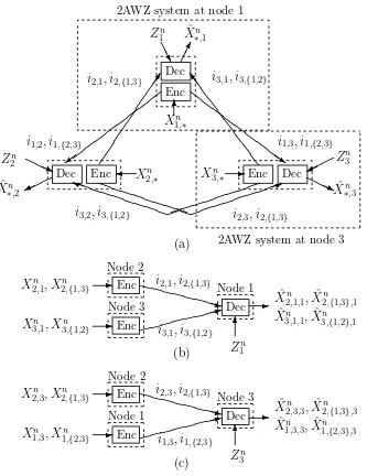
Starting with the WZ system of Figure 3.1(d), consider adding a third node that describes a new sourceX3,1 to the decoder at node 1. This creates a 2A system with side information at the decoder (a 2AWZ system), as depicted in Figure 3.3. There are at least two options for updating the code. In the first, the encoder at node 2 stays the same, the decoder retains its previous codebook for jointly decoding (î2,1, Z1), and a new conditional codebook for decoding î3,1, conditioned on (î2,1, Z1), is trained. This greedy approach keeps the previous system intact and simply adds new components. However, the correlation between X3,1 and X2,1 is exploited only in the decoding of X3,1 and not X2,1. Optimally exploiting the correlation so as to minimize the Lagrangian cost (3.2) requires a second, global approach, in which the original WZ codebook is extended to jointly decode all three inputs (î2,1,î3,1, Z1). For this, the whole system must be retrained.

On source coding for networks