Exploratory differential gene expression analysis in microarray experiments with no or limited replication

(1)

en

t

re

v

ie

w

s

re

ports

de

p

o

si

te

d r

e

sea

rch

refer

e

d

re

sear

ch

interacti

o

ns

inf

ormation

experiments with no or limited replication

Alexander V Loguinov

*

_{, I Saira Mian}

†

_{and Chris D Vulpe}

*

Addresses: *_{Department of Nutritional Sciences and Toxicology, University of California at Berkeley, Morgan Hall, Berkeley, CA 94720, USA.} †_{Life Sciences Division, Lawrence Berkeley National Laboratory, Cyclotron Road, Berkeley, CA 94720, USA.}

Correspondence: Alexander V Loguinov. E-mail: [email protected]. Chris D Vulpe. E-mail: [email protected]

© 2004 Loguinov et al.; licensee BioMed Central Ltd. This is an Open Access article: verbatim copying and redistribution of this article are permitted in all media for any purpose, provided this notice is preserved along with the article's original URL.

Exploratory differential gene expression analysis in microarray experiments with no or limited replication

We describe an exploratory, data-oriented approach for identifying candidates for differential gene expression in cDNA microarray exper-iments in terms of α-outliers and outlier regions, using simultaneous tolerance intervals relative to the line of equivalence (Cy5 = Cy3). We demonstrate the improved performance of our approach over existing single-slide methods using public datasets and simulation studies.

Abstract

We describe an exploratory, data-oriented approach for identifying candidates for differential gene expression in cDNA microarray experiments in terms of

α

-outliers and outlier regions, using simultaneous tolerance intervals relative to the line of equivalence (Cy5 = Cy3). We demonstrate the improved performance of our approach over existing single-slide methods using public datasets and simulation studies.

Background

Multiple studies validate the utility of cDNA microarrays for comparing relative mRNA transcript levels between different biological samples. Both the biological systems under study and the technology itself contribute to the variability within and between microarrays [1-11]. A fundamental question is determining which of the potentially tens of thousands of genes assayed have transcript levels that differ significantly in the two samples. Experimental designs utilizing many levels of replication improve the ability to identify differentially-expressed genes [2-12]. However, the vast majority of studies utilize no or limited replication due to practical considera-tions of cost and feasibility. Thus, statistical techniques are needed for cDNA microarray studies with constraints on rep-lication. A common strategy is to equate differentially-expressed genes with those genes having a ratio of hybridiza-tion intensity values greater, or less, than some user-defined threshold [13,14], such as two-fold change.

We describe a new approach for identifying differentially expressed gene candidates in cDNA microarray experiments without replication or with limited replication. We illustrate its utility by applying it to published data and demonstrate its

advantages over current approaches. Microarray datasets are comprised of pairs of processed fluorescent intensity values,

background corrected and normalized, for each of the N

genes on the microarray. We discuss a model for such data in

which the log₂(Cy5) and log₂(Cy3) values are linearly related

and are samples drawn from a bivariate normal population 'contaminated' with outliers (see detailed definitions of the outlier-generating model in Methods) and possibly distorted due to heteroscedasticity. In a contaminated bivariate normal distribution, the main body of data is a sample from a bivari-ate normal distribution and constitutes the regular observa-tions. The dataset also contains non-regular observations, 'outliers' or 'contaminants', which represent systematic devi-ations that, as we describe below, are candidates for differen-tial expression. We check these underlying assumptions by applying exploratory data analysis tools (scatter plots with tolerance ellipses, Quantile-Quantile normal plots (QQNPs) with simulation envelopes and boxplots for residuals) to sim-ulated and empirical datasets.

We formulate our method in terms of an α-outlier-generating

model and outlier regions [15,16]. In a scatter plot of suitably

normalized log₂(Cy5) versus log₂(Cy3) intensity values the

Published: 1 March 2004 Genome Biology 2004, 5:R18

Received: 24 June 2003 Revised: 1 December 2003 Accepted: 11 December 2003 The electronic version of this article is the complete one and can be

(2)

majority of data points lie in the vicinity of the line of

equiva-lence (Cy5 = Cy3). The line of equivalence can be estimated

using a robust linear regression estimator and normalizing data by the regression fit making slope = 1 and intercept = 0.

We subtract the fit from data to compute residuals [log₂(Cy5)

- log₂(Cy3)] which represent the vertical distances from the

line of equivalence to the data points and are equivalent to the

log-transformed ratios log₂(Cy5/Cy3). After these steps, we

apply robust scatter plot smoothers to quantify and take into account the distortion of the data, if any, by heteroscedastic-ity. Data points far from the line of equivalence, 'outliers', are considered to be of greatest interest since they correspond to genes having noticeably different hybridization intensity val-ues. An outlier could represent one of five circumstances: a gene with higher individual variability than the majority of genes; an outlier by chance; a sporadic technical or biological outlier; a systematic technical outlier (due to, for example, heteroscedasticity); or a systematic biological outlier due to differential expression. We assume that the further away from the line of equivalence an outlier is located, the more likely that it is genuinely 'up-' or 'down-regulated'. We com-pare our approach with some existing single-slide methods [13,14,17-20] and demonstrate that it works well in practice.

Results

We examined 10 published cDNA microarray experiments

that compared 6,295 transcript levels in wild-type

Saccharo-myces cerevisiae and single gene deletion mutants pertinent to copper and iron metabolism [18]. The deleted genes were mac1/YMR021C (experiment number 96), cin5/YOR028C

(26), cup5/YEL027W (36), fre6/YLL051C (64), sod1/

YJR104C (162), spf1/YEL031W (163), vma8/YEL051W

(189), yap1/YML007W (195), yer033c (214) and ymr031c

(250).

Exploratory data analysis supports model for cDNA microarray data

We used exploratory data analysis tools to assess the assump-tions underlying our method. We assume that biological and technical noise results in the majority of the measured expression levels changing randomly, independently,

non-directionally and by a small amount. Thus, the log₂(Cy3) and

log₂(Cy5) variables in cDNA microarray data should be

line-arly related and come from a contaminated bivariate normal distribution, possibly distorted due to heteroscedasticity.

Using each tool, we compared the observed mac1 data and

datasets simulated as samples from a bivariate normal distri-bution with parameters corresponding to robust estimates of the location and variance-covariance matrix. Figure 1 shows

concentration ellipses and QQNP for log₂(Cy5/Cy3) values

for empirical and simulated datasets.

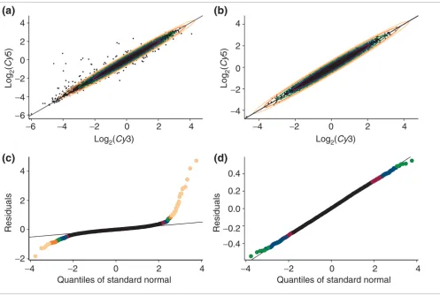
The log₂(Cy5) versus log₂(Cy3) scatter plots and

concentra-tion ellipses (Figure 1a,1b) provide a visual assessment of

bivariate normality. The distribution of the mac1 empirical

data is similar to the simulated ('ideal') bivariate normal

pop-ulation except for the presence of strong outliers. The mac1

data include significantly more unexpected events than might be expected for a sample from a bivariate normal population.

The QQNP for residuals (log₂(Cy5/Cy3)) compares the

quan-tiles of the empirical data with the quanquan-tiles of the standard

normal distribution (Figures 1c,d). The mac1 simulated data

points lie along a straight line (the line for the standard nor-mal distribution) except for some heavy tails due to finite

sample size (Figure 1d). The empirical mac1 data points

(Fig-ure 1c) also conform to a normal distribution except for longer tails (increased incidence of outliers and possible het-eroscedasticity). Examination of the empirical data using

exploratory data analysis tools supports our premise that the

log-transformed channel intensities (log₂(Cy3) and

log₂(Cy5)) are linearly related and come from a contaminated

bivariate normal distribution possibly distorted with heteroscedasticity.

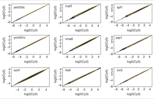
The other nine datasets show a similar pattern (Figures 2,3,4,5,6,7,8,9,10). Figure 2 shows nine scatter plots with tol-erance ellipses for the empirical log-transformed normalized channel intensities. There are strong bivariate outliers and differential gene expression candidates will be represented by

Y-outliers. A data point which is an X-outlier or Y-X-outlier

probably represents a technical gross error. Figure 3 repre-sents scatter plots for simulated data produced using robust estimates of location and scale parameters for the corre-sponding empirical datasets. A 99.99% tolerance ellipse cov-ers the simulated data points with no outlicov-ers. Figure 4 displays results after outlier removal from the empirical data using a simple cut-off and ignoring heteroscedasticity, if any. The majority of data points look like regular observations sampled from a bivariate normal population.

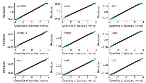
Ordinary QQNP results represented in Figures 5,6,7 are a dif-ferent view of the data shown in Figures 2,3,4, comparing empirical, or simulated, quantiles with quantiles of the stand-ard normal distribution. Outlying observations are all in the heavy tails. Figure 6 demonstrates the absence of strong out-liers in the simulated data but heavy tails still persist due to finite sampling. Figure 7 shows that after the outlier removal, the main body of data ('regular observations') may be reason-ably approximated with a normal distribution. Simulation envelopes for the QQNP support this conclusion, see text below.

(3)

comm

en

t

re

v

ie

w

s

re

ports

refer

e

d

re

sear

ch

de

p

o

si

te

d r

e

se

a

rch

interacti

o

ns

inf

o

rmation

other scatter plots based on datasets from Hughes et al. [18]).

Such a local non-linearity could be removed by applying a lowess-based normalization with appropriate smoothing parameters. The source of the systematic deviation is not known.

Detection of residual heteroscedasticity

In microarray data, the variance of residuals (log₂(Cy5/Cy3))

is not a constant (homoscedasticity) but rather varies

(heter-oscedasticity) with intensity level (log₂(Cy5Cy3)/2 or

log₂(Cy3) or log₂(Cy5)). The presence of residual

hetero-scedasticity argues strongly against arbitrary threshold meth-ods to identify candidates for differential expression [10,11,19,21-24]. Approaches for assessing the heterogeneity of residual variance [10,11,25,26] include graphical, paramet-ric and non-parametparamet-ric methods. Here, we use non-paramet-ric regression smoothing in 'absolute residuals versus

log₂(Cy3)' scatter plots to quantify residual variance. We

compared S-plus/R supsmu (super smoother) and lowess

(robust locally weighted regression) with other methods (scatter plots with tolerance ellipses, QQNPs with simulation envelopes, boxplots for residuals) and found that our regres-sion smoother approach for absolute residuals performs well.

We used these smoothing methods to assess heteroscedastic-ity in the following way: grouping data into subsets of equal size and then applying regression smoothers to the median

absolute residual in each group against median of log₂(Cy3)

for that group [25]; same as this method but using boxplot for each group. One benefit of the latter approach is the fact that it can be used directly not only for residual diagnostics but also to take into account heteroscedasticity and estimate the number of candidates for differential gene expression. We also used Spearman rank correlation coefficients of the

abso-lute residuals versus log₂(Cy3) to check the smoothing-based

methods for consistency: positive values indicate increasing residual variance, negative ones indicate decreasing variance [25].

[image:3.612.57.554.85.419.2]

Visual tests of the underlying assumptions Figure 1

Visual tests of the underlying assumptions. Five concentration ellipses for (a) the standardized mac1 dataset and (b) for a Monte Carlo simulated dataset with the same parameters of location and variance-covariance matrix (we used robust versions the location and scale estimators) as in mac1 data. The tolerance ellipses cover 90% (red), 95% (blue), 99% (green), 99.9% (orange) and 99.99% (light orange) portions of the standard normal distribution to assist in visually testing the assumption of contaminated bivariate normality. QQNP of residuals for (c) mac1 dataset and (d) for the corresponding Monte Carlo simulated dataset for comparison with (a) and (b). Outlying points are given in different colors in accordance with STIs in Figure 19b.

Log₂(

Cy

3)

Log

2

(

Cy

5)

Log₂(

Cy

3)

Log

2

(

Cy

5)

Quantiles of standard normal Quantiles of standard normal

Residuals Residuals

−4 −2 4

2

0

−2 4

2

0 −4 −6

−6 −4 −2 0 2 4 −4 −2 0 2 4

−4 −2 0 2 4 −4 −2 0 2 4

−2 4

2

0

−0.4 −0.2 0.0 0.2 0.4

(a)

(b)

(4)

We show an example of the results in Table 1 and Figures

11,12,13,14,15,16 for the cup5 dataset. Figure 11 demonstrates

the dependence between smoothed absolute residuals and

smoothing parameters for supsmu and lowess procedures. As

expected, supsmu procedure is more sensitive to prominent

outliers in low intensity regions because it uses an automati-cally adjusted variable span. Prominent outliers in the low

intensity area are both Y- and X-outliers and should be

dis-carded. For the majority of cup5 data, supsmu and lowess

generate similar results. Figure 12 shows supsmu and lowess

smoothing for 20 median-based sequential intervals of equal size and using different values of smoothing parameters at

'higher' resolution. Figure 13 does the same using cup5 data

in background. Figures 14 and 15 show boxplots for residuals

using 10 and 20 equal size sequential intervals, respectively. They confirm the presence of heteroscedasticity as well. Box-plots for residuals with 20 subgroups of equal size using

±3IQR-based upper and lower extremes give an estimate for

k = 75. This estimate is close to k = 61 identified by adjusted

supsmu-based 99.998% simultaneous tolerance intervals (STIs) (Table 2). The difference in the estimates (14, or about

19%) can be explained by the fact that the ±3IQR rule

gener-ates about a 99.995% two-sided tolerance interval for a nor-mally distributed population, while for a sample of finite size

the corresponding upper and lower tolerance limits are wider (compare Equations 8 and 9) to cover 99.998% per residual group. Figure 16 is a smoothed version of Figure 14 using supsmu and lowess procedures for 3IQR-based extreme limits.

Statistical significance of outliers: ordinary and smoothed STIs

Our method equates contaminants of bivariate normal distri-butions (outliers) with candidates for differential expression. The outlier identification method has been developed previ-ously for other applications [16,27,28]. We employ an

approach based on the perspective of α-outliers and outlier

regions [15,16]. In this approach, a point above the line of

equivalence (that is, Cy3 = Cy5) is viewed as a candidate for

an up-regulated gene, one below the line as a down-regulated gene and one in the vicinity of the line as an unchanged gene. Intuitively, points further away from the line - stronger out-liers - are most likely to represent differentially-expressed genes. In other words, the probability that the observed dif-ference in transcript level between the two samples might have arisen by chance decreases. To quantify these qualitative ideas, we applied statistical criteria to decide when points might result from no actual difference in expression (for

5)

−8 −6 −4 −2 0 2 4

yer033c

cup5

spf1

ymr031c

vma8

yap1

sod1

fre6

cin5

−6 −2 0 2 4

−10 −6 −2 2 4

−8 −4 0 2 4

−6 −2 0 2 4

−10 −6 −2 2 4

−6 −2 0 2 4

−8 −4 0 2 4

(5)

comm en t re v ie w s re ports refer e e d re sear ch de p o si te d r e se a rch interacti o ns inf o rmation

example, due to random fluctuations) versus those corre-sponding to genuine differential expression. We used a

general α-outlier model for residuals (log-transformed

nor-malized ratios) to identify candidates for differential expression.

In order to estimate the statistical significance of outliers, we used simultaneous tolerance intervals (STIs) based on Scheffé simultaneous confidence principles [29,30]. This approach guarantees a desired confidence level across the

whole range of the predictor variable X = log₂(Cy3), log₂(Cy5)

or log₂(Cy3Cy5)/2 and for all P = 100%q(the portion of the

normal distribution covered by a certain STI, see Methods). We modified the approach using robust regression smoothers (supsmu or lowess) to approximate an unknown relationship,

s2 ₌_F₍_X_{), between residual variance and intensity. Five STIs}

for the mac1 empirical and simulated datasets are shown

(Figure 17a,b). For ordinary STIs, random fluctuations are seen to contribute to data points located away from the line of equivalence. However, the empirical data contain more and stronger outliers than the simulated data (Figure 17b). The five ordinary STIs were constructed under the assumption

that the residual variance is constant (homoscedasticity) across the entire range of values for the predictor variable. We

notice that for a large sample size (N = 6068, see Methods)

ordinary STIs appear as straight lines (for small and moder-ate datasets they appear as hyperbolas; see Equations 2, 8,

and 9 in Methods). Figure 17c shows residuals (log₂(Cy5/

Cy3)) as a function of X = log₂(Cy3) for the empirical mac1

dataset. This plot and residual plots for other nine experi-ments (Figure 18) reveal that residual variance is not a con-stant (heteroscedasticity). Residual variance is commonly

high for small values of X_i; it decreases to a minimum and

may increase for large values of X_i, that is, the empirical

dependence appears hyperbolic. We account for the hetero-scedasticity by the use of smoothed STIs (Figure 17d). Accord-ingly, smoothed STIs appear as curves that are wider at low

and high X_ivalues. Therefore, for a given portion of the

nor-mal distribution covered by a certain STI, points with X_i

val-ues at either extreme are further away from the line of equivalence.

For mac1, the width of the smoothed STIs is somewhat

greater at low intensities compared to those at high

[image:5.612.57.555.87.411.2]

Overlay of concentration ellipses for the bivariate standard normal on simulated data Figure 3

Overlay of concentration ellipses for the bivariate standard normal on simulated data. Scatter plots of nine simulated datasets (generated as random samples from a bivariate normal population) with overlaid concentration ellipses for the standard bivariate normal distribution (see Figure 1 for the portions captured). Channel intensity values were log(base 2)-transformed, normalized and standardized.

log₂(

Cy

3)

log

2

(

Cy

5)

5)

yer033c

cup5

spf1

ymr031c

vma8

yap1

sod1

fre6

cin5

−4 −2 0 2 4

(6)

intensities. In the mid-range of X_ivalues, smoothed STIs lead to intervals that are narrower than ordinary STIs that do not consider heteroscedasticity. Therefore, candidates for differ-entially-expressed genes are more likely to be identified in the

middle range of X_ivalues and are less likely to be defined at

the extremes.

We evaluated the lowess- and supsmu-smoothing procedures

by applying them to a simulated dataset taken from an 'ideal' bivariate normal population with the same parameters as the

empirical mac1 dataset. The robust scale estimates using the

Huber τ-estimator for scale, supsmu- and lowess-based scale

estimators are shown in Figure 19a. The smoothed scale esti-mators generate approximately straight lines parallel to the

Huber τ-scale estimator.

Adjusted STI

An adjustment for Gaussian efficiency is necessary for the application of robust estimators [31] such as those we use for outlier identification in the presence of heteroscedasticity. We therefore adjust smoothed STIs to improve their accu-racy. We calculate an adjustment constant (scale factor) to

compensate for the difference between the Huber τ-estimator

for scale and supsmu- or lowess-based scale estimators (see

Methods for details). The adjusted constant is used as a scale factor for the smoothed STIs for empirical data. Adjusted smoothed STIs are shown in Figure 18 and Figure 19b. The dramatically different STIs amongst the ten datasets reflect their individual patterns of residual variance and demon-strate the necessity of tailored analysis of a dataset.

Candidates for differential expression

We identify candidates for differential expression by using

STIs containing the P = 100(1 - α) portion of normal

distribu-tion covered with probability at least 1- γ (see Methods). For

mac1, no simulated data lies outside the 99.998% ordinary

STIs (γ-level = 0.0001) suggesting that empirical data points

outside the corresponding adjusted smoothed supsmu-based

STIs are good candidates for differentially-expressed genes.

For the mac1 analysis (Table 3), 41 candidate genes for

up-regulation and 20 candidates for down-up-regulation are

identi-fied using a 99.998% (γ-level = 0.0001) adjusted supsmu

-based STI. For the ten datasets examined, up to approxi-mately 2% of the genes were candidates for differential

[image:6.612.59.557.87.407.2]

Overlay of concentration ellipses for the bivariate standard normal on real data with prominent outliers removed Figure 4

Overlay of concentration ellipses for the bivariate standard normal on real data with prominent outliers removed. Scatter plots of nine datasets from Hughes et al. [18] after outlier removal with concentration ellipses for the standard bivariate normal distribution (see Figure 1 for the portions captured). Two-sided 99.9% cut-off and robust measure of scale (median absolute deviation) for residuals were used to identify outliers. Channel intensity values were log(base 2)-transformed, normalized and standardized.

log2(Cy3)

log2(Cy5)

−6 −4 −2 0 2 4

−6 −4 −2 0 2 4 −6 −4 −2 0 2 4

−6 −4 −2 0 2 4

−6 −4 −2 0 2 4 log2(Cy3)

log2(Cy5)

−6 −4 −2 0 2 4

log2(Cy3)

log2(Cy5)

−8 −6 −4 −2 0 2 4

log2(Cy3)

log2(Cy5)

log2(Cy3)

log2(Cy5)

log2(Cy3)

log2(Cy5)

log2(Cy3)

log2(Cy5)

−4 −2 0 2 4

log2(Cy3)

log2(Cy5)

log2(Cy3)

log2(Cy5)

cin5 fre6

sod1

yap1 vma8

ymr031c

spf1 cup5

yer033c

−6 −2 0 2 4

−4 0 2 4

−6 −2 0 2 4

−6 −2 0 2 4 −8 −4 0 2 4

−8 −4 0 2 4

(7)

comm

en

t

re

v

ie

w

s

re

ports

refer

e

d

re

sear

ch

de

p

o

si

te

d r

e

sea

rch

interacti

o

ns

inf

ormation

expression (see Table 2, Table 3 and Table 4 for mac1 data

and a comparative summary table for all ten datasets in Addi-tional data). Overall, adjusted smoothed STIs provide a better balance between sensitivity and specificity across the whole

range of predictor variable values (log₂(Cy3)) and are thus

more reliable than ordinary STIs. The approach takes into consideration multiplicity of comparisons, variation in the experimental response around the line of equivalence (or around zero for residuals) and intensity dependent variation in residual variance.

Differential expression in a single cDNA microarray: adjusted smoothed STIs and existing methods

We compared the adjusted smoothed STI technique for iden-tifying differentially-expressed genes with other methods for single cDNA microarray data [13,14,17-19]. Within the frame-work of outlier detection analysis, the primary difference amongst these methods is the means used to define statistical intervals (see Discussion for the details of each model). In the

arbitrary ratio approach, Y_i/X_i= log₂(Cy5/Cy3) = r_idefines a

gene i as being differentially expressed if r_i>t where t is a

user-defined threshold [13,14,17]. The most frequently used

value t corresponds to residuals of -1 (two-fold down) and 1

(two-fold up). Figure 20 compares differential expression in three different experiments using a ratio threshold and

adjusted supsmu-based STIs. For t = ± 1, any gene outside

this cut-off would be deemed as up- or down-regulated. How-ever, employing the criterion of genes higher than the

99.998% (γ-level = 0.0001) adjusted supsmu-based STIs

would yield additional candidates for differential expression.

Although t = ± 1 seems more conservative for these datasets,

it may be overly liberal for others.

Hughes et al. [18] developed an error model that made use of

additional information about the variability of each gene based on 63 'same versus same' control experiments. Figure

21a and Table 4 compare differential expression in the mac1

data as defined using the 'gene-specific' error model [18] and

adjusted supsmu-based STIs. As we discuss below, some

genes which were identified as differentially expressed using

our adjusted supsmu-based STIs were not identified by the

error model [18]. Our approach with four other models [17,19,20] (see also Discussion) in an outlier detection frame-work is compared in Figure 21a,b.

[image:7.612.55.553.85.406.2]

QQNP for real data: residuals of nine datasets from Hughes et al. [18] Figure 5

QQNP for real data: residuals of nine datasets from Hughes et al. [18]. Channel intensity values were log(base 2)-transformed and normalized. Compare with Figure 18 (colors for outliers match the tolerance band colors).

Quantiles of standard normal

Residuals

−4 −2 0 2 4 −4 −2 0 2 4 ₋4 −2 0 2 4

−4 −2 0 2 4 −4 −2 0 2 4 −4 −2 0 2 4

yer033c cup5 spf1

ymr031c vma8 yap1

sod1 fre6 cin5

−1 0 1

−6

−2 2 4 6

−3

−1 1 2

−6

−2 2 4 6

−4 0 2 4

−6

−2 2 4 6

−4

−2 0 1 2

−6

−2 0 2 4

−6

−4

(8)

In general, our adjusted smoothed STI method generates nar-rower bands in the mid-range of gene expression levels and

broader bands in low and higher intensity areas. For mac1,

the bands for Newton et al.'s method [19] and our method

appear similar qualitatively. The STI-based measure of statis-tical significance takes into consideration the unique features and properties of empirical microarray datasets.

Simulation studies

We carried out simulation studies using sample parameter

estimates from the mac1 dataset to assess the performance of

each of the single-slide methods. We created artificial data-sets with 100 candidates (outliers) for differential expression.

We simulated k = 100 non-regular observations and N-k =

6,068-100 = 5,968 regular observations (the main body of non-differentially-expressed genes). A random component was added to each outlier value using standard normal distri-bution with variance dependent on intensity. This set of 100 represents the 'true' outliers due to 'differential expression'. We simulated heteroscedasticity present in many datasets by including intensity-dependent variability in the low and high intensity levels for both non-regular and regular data points. We then compared the performance of each method to iden-tify candidates for differential expression in multiple repeat runs of the simulation. (R code and data used for the simula-tions can be obtained from the authors upon request.) Figure

22 shows a plot of the simulated data with true outliers shown in red. We compared the performance of several different sin-gle-slide methods at ten 'cut-off' levels of relatively equivalent

stringency as shown in Table 5 (except for Chen et al. [17]

which use only two levels of significance). We compared PPV (positive predictive value), NPV (negative predictive value), sensitivity, specificity and likelihood ratios at each cut-off for each method (please see definitions of the test accuracy meas-ures in [32] and in Additional data). We plotted these results in Figure 23 as a receiver operating characteristic (ROC) curve, a PPV curve, and a likelihood ratio curve. These results clearly demonstrate that our method outperforms existing single-slide methods with improved positive predictive val-ues, likelihood ratio and higher ROC curves (greater area under the curve). These improved performance differences are most apparent at the most stringent significance levels which are likely to be most relevant in the context of multiple comparisons.

Comparison of biological significance of mac1 results

The effects of the mac1∆ on the metabolism and gene

expres-sion in yeast are well documented. The absence of the Mac1p, a copper responsive transcription factor, results in down-reg-ulation of copper uptake transporters and subsequent copper deficiency [33-36]. Copper is required for Fet3p which in turn is necessary for iron uptake in yeast. As a consequence,

[image:8.612.58.556.88.371.2]

QQNP for residuals of nine simulated datasets (generated as random samples from a normal population) Figure 6

QQNP for residuals of nine simulated datasets (generated as random samples from a normal population). Channel intensity values were log(base 2)-transformed and normalized. Compare with Figure 18 (colors for outliers match the tolerance band colors).

Residuals

−4 −2 0 2 4

−0.04 0.0 0.04

−4 −2 0 2 4 ₋4 −2 0 2 4

−4 −2 0 2 4 −4 −2 0 2 4 −4 −2 0 2 4

yer033c cup5 spf1

ymr031c vma8 yap1

sod1 fre6 cin5

−0.06 0.0 0.06

−0.04 0.0 0.04

−0.06 0.0 0.04

−0.04 0.02

−0.06 0.0 0.04

−0.04 0.02

(9)

comm

en

t

re

v

ie

w

s

re

ports

refer

e

d

re

sear

ch

de

p

o

si

te

d r

e

sea

rch

interacti

o

ns

inf

ormation

copper deficiency results in secondary iron deficiency [37,38]. Iron deficiency leads to activation of iron responsive transcription factors, Aft1p and Aft2p, which induce tran-scription of a host of genes encoding proteins involved in iron uptake [39]. The identification of up-regulation of these tar-get genes provides a reasonable biological standard for com-paring the performance of the different methods. In addition, down-regulation of Mac1p targets might be expected in a

mac1∆. In Table 4, we present a comparison of the methods at

relatively equivalently high levels of stringency for likely Aft1/ 2p and Mac1p targets present on the arrays and identified by at least one method as differentially expressed. We also include the two-fold cut-off for comparison. A total of 13

genes were not identified as up-regulated by Hughes et al.

Two genes previously identified as a Mac1p target (YFR055W) [40] or down-regulated in mac1∆ (CTT1) [33] and MAC1 itself were not identified by the Hughes et al. method. While identifying many of the Aft1/2p targets

excluded by Hughes et al., the other two methods did not

identify MRS4 or SMF3, which are regulated in response to

iron deficiency, nor did they identify YFR055W and CTT1 as

down-regulated. We suggest that these results provide some biological validation of our approach and indicate increased performance of our method over the other methods at

stringent significance levels - necessary given the multiplicity of comparisons.

Discussion

Multiple replications in the design of reagents (multiple spot-ting of each gene on a microarray) and experimental approach (multiple replicates of each hybridization) provide the soundest approach to confirm differential expression of genes (see, for example, [2-12]). However, experimental real-ities such as limited samples (for example, tumor specimen), a large number of samples (for example, time course experi-ments) and experimental cost have resulted in the vast major-ity of published cDNA microarray studies using limited or no replication. Several methods currently exist for the analysis of data from experiments with limited or no replication. Unfor-tunately, real microarray data generally violate the assump-tions underlying these methods.

Limitations of underlying assumptions of current single -slide methods

Chen et al. [17] assumed that raw non-normalized and non

log-transformed Cy5 and Cy3 intensities (raw intensities) are

drawn from independent normal populations with common

[image:9.612.54.555.85.380.2]

QQNP for residuals of nine datasets from Hughes et al. [18] after prominent outlier removal Figure 7

QQNP for residuals of nine datasets from Hughes et al. [18] after prominent outlier removal. Two-sided 99.9% region and robust measure of scale (median absolute deviation) for residuals were used to remove outliers. Channel intensity values were log(base 2)-transformed and normalized. Compare with Figure 18 (colors for outliers match the tolerance band colors).

Residuals

−4 −2 0 2 4 −4 −2 0 2 4 −4 −2 0 2 4

cin5 fre6

sod1

yap1 vma8

ymr031c

spf1 cup5

yer033c

−0.2 0.0 0.2

−0.6 0.0 0.4

−0.2 0.2

−0.6 0.0 0.4

−0.4 0.0 0.4

−0.6 0.0 0.4

−0.4 0.0 0.4

(10)

coefficient of variation. An asymmetric density function for raw ratios was derived. This results in asymmetric bands with the identification of more up-regulated than down-regulated genes irrespective of the dataset (compare Figure 4 in [19] and Figure 7 in [8]).

Newton et al. [19] assumed that because raw Cy5 and Cy3

intensities are always positive they can be considered as observations from a Gamma distribution with the same

coef-ficient of variation (if Cy3 and Cy5 are independent, their

joint distribution is a bivariate Beta distribution). Hierarchi-cal Gamma-Gamma and Gamma-Gamma-Bernoulli models were formulated in which the posterior odds of change in

expression were an additive (Cy5 + Cy3) and multiplicative

(Cy5Cy3) functions of intensity. Contours of the posterior

odds in (X≡ log(Cy3), Y≡ log(Cy5)) scatter plots were used to

identify differentially-expressed genes. In practical situations, it may be difficult to determine if data are log-nor-mal or Gamma [41] but we argue that the former is more real-istic for microarray data because the combination of biological and experimental noise results in the majority of the measured expression levels changing randomly,

independently, non-directionally and for those changes to be small. The central limit theorem would therefore predict bivariate normality for the majority of log-transformed spot intensity values.

Sapir and Churchill [20] compute the posterior probability of differential expression using a mixture of orthogonal

residuals derived from ordinary least squares regression of (X

≡ log₂(Cy3), Y≡ log₂(Cy5)). The approach assumes that

differ-entially-expressed genes are drawn from populations with unknown distributions approximated with uniform distribu-tions. This mixture model approach assumes that all outliers

(k non-regular observations) follow the same distribution D₀

= D₁= ... = D_k. Under a mixture model, contaminants are less

separated from the regular observations than when using Fer-guson-type model [16]. The method used to obtain orthogo-nal residuals in this approach is not resistant to outliers [42] and is redundant because the use of log-transformed ratios

log₂(Cy5/Cy3) assumes normalization by linear regression to

enforce slope equal to 1 and intercept equal to 0 (compare [8]). This approach does not take into consideration residual

heteroscedasticity. Similarly, Yue et al. [1] described a

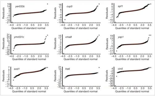
[image:10.612.56.558.86.398.2]

QQNP with simulation envelopes (based on 1,000 random samples from a normal population) for residuals of nine datasets from Hughes et al. [18] Figure 8

QQNP with simulation envelopes (based on 1,000 random samples from a normal population) for residuals of nine datasets from Hughes et al. [18]. Channel intensity values were log(base 2)-transformed and normalized. The envelopes are depicted as dashed red lines.

−4.0 −2.5 −1.0 0.5 2.0 3.5

Residuals

−4.0 −2.5 −1.0 0.5 2.0 3.5

Residuals

−4.0 −2.5 −1.0 0.5 2.0 3.5

Residuals

−4.0 −2.5 −1.0 0.5 2.0 3.5

Residuals

−4.0 −2.5 −1.0 0.5 2.0 3.5

Residuals

−4.0 −2.5 −1.0 0.5 2.0 3.5

Residuals

−4.0 −2.5 −1.0 0.5 2.0 3.5

Residuals

−4.0 −2.5 −1.0 0.5 2.0 3.5

Residuals

−4.0 −2.5 −1.0 0.5 2.0 3.5

Residuals

yer033c cup5 spf1

ymr031c vma8 yap1

sod1 fre6 cin5

−21 −16 −11−6 −14 9 14 19

−19 −14−9 −41 6 11 16

−13 −10− 7 −4 −1 2 5 8

−32 −25 −18 −11-4 3 10 17 24 31

−17 −13−9 −5 −13 7 11 15

−23 −17 −11− 5 1 7 13 19

−17 −14 −11−8 −5 −21 4 7

−33 −27 −21 −15−9 −33 9 15 21

(11)

comm en t re v ie w s re ports refer e e d re sear ch de p o si te d r e se a rch interacti o ns inf o rmation

method based on parametric two-sided tolerance intervals for ratios. This approach does not consider residual hetero-scedasticity and the multiplicity of comparisons.

Hughes et al. [18] performed 63 control 'same versus same'

hybridizations in addition to 300 'treatment versus control' cDNA microarray experiments, many in duplicate. They fil-tered candidates for differential expression on the basis of the information about individual variability in expression levels, and genes with unusually high variation were discarded (Fig-ure 21a). One possible drawback is the assumption that the

expression variance is the same in both samples. Hughes et

al. [18] quantified residual heteroscedasticity using weighted

location and scale estimators for 'same versus same' repli-cates. Their method used non-robust versions for the estima-tors - consequently the location estimates may have a bias and the scale estimates would be significantly inflated in the pres-ence of outliers [43]. In addition, since this method uses extensive 'same versus same' hybridizations, it cannot be con-sidered to be a single-slide method.

Advantages of

α

-outlier model and outlier identification method

In this work, we have described a post hoc (data-oriented)

method, which makes fewer assumptions about the nature of the data, tests the assumptions to ensure their validity and produces computationally reasonable results. We showed that a reasonable model is one where the processed fluorescent intensity values are samples drawn from a bivari-ate normal population contaminbivari-ated with outliers and possi-bly distorted due to heteroscedasticity. After a normalization by a robust linear regression fit to make slope equal to 1 and intercept equal to 0, in general, most data points in the

log₂(Cy5) versus log₂(Cy3) scatter plot lie close to the line of

equivalence (log₂(Cy5) = log₂(Cy3)) while a limited number

of data points, outliers, lie outside the vicinity. The outliers are good candidates for differentially-expressed genes. The further an outlier is located from the line of equivalence the more likely it is to represent a systematic outlier rather than a

chance observation. The α-outlier-generating model

approach for identifying differentially expressed gene

[image:11.612.58.554.87.404.2]

QQNP with simulation envelopes for Monte Carlo simulated data Figure 9

QQNP with simulation envelopes for Monte Carlo simulated data. QQNP with simulation envelopes (based on 1,000 random samples from a normal population) for residuals of nine simulated datasets (generated as random samples from a normal population). Channel intensity values were log(base 2)-transformed and normalized. The envelopes are depicted as dashed red lines.

−4.0 −2.5 −1.0 0.5 2.0 3.5 Quantiles of standard normal

Res

id

u

a

ls yer033c cup5 spf1

ymr031c vma8 yap1

sod1 fre6 cin5

−5 −3 −1 1 3 5

Res id u a ls −5 −3 −1 1 3 5

(12)

[image:12.612.59.557.87.401.2]

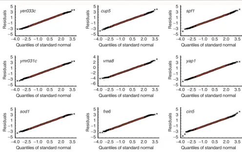
QQNP with simulation envelopes (based on 1,000 random samples from a normal population) for residuals of nine datasets from Hughes et al. [18] after prominent outlier removal

Figure 10

QQNP with simulation envelopes (based on 1,000 random samples from a normal population) for residuals of nine datasets from Hughes et al. [18] after prominent outlier removal. Two-sided 99.9% cut-off and robust measure of scale (median absolute deviation) for residuals were used to remove outliers. Channel intensity values were log(base 2)-transformed and normalized. The envelopes are depicted as dashed red lines.

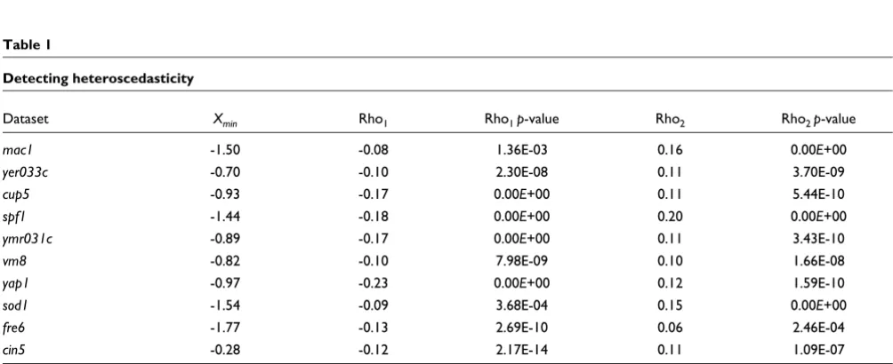
Table 1

Detecting heteroscedasticity

Dataset X_min Rho₁ Rho₁p-value Rho₂ Rho₂p-value

mac1 -1.50 -0.08 1.36E-03 0.16 0.00E+00

yer033c -0.70 -0.10 2.30E-08 0.11 3.70E-09

cup5 -0.93 -0.17 0.00E+00 0.11 5.44E-10

spf1 -1.44 -0.18 0.00E+00 0.20 0.00E+00

ymr031c -0.89 -0.17 0.00E+00 0.11 3.43E-10

vm8 -0.82 -0.10 7.98E-09 0.10 1.66E-08

yap1 -0.97 -0.23 0.00E+00 0.12 1.59E-10

sod1 -1.54 -0.09 3.68E-04 0.15 0.00E+00

fre6 -1.77 -0.13 2.69E-10 0.06 2.46E-04

cin5 -0.28 -0.12 2.17E-14 0.11 1.09E-07

Use of Spearman rank correlation for absolute residuals to detect heteroscedasticity [25] in ten datasets from Hughes et al. [18]. Empirical hyperbolas (here they are based on supsmu smoother) have minima around sample means. As a result, we use two subintervals to compute Spearman rank correlation coefficient: from minus infinity to X_min(log₂(Cy3) axis) and from X_minto plus infinity. We note that sign of Spearman rank correlation always coincides with the sign of first derivative for empirical hyperbolas at a given subinterval (compare Figure 20). Rho₁, Spearman coefficient of rank correlation for the former subinterval; Rho₁p-value, p-values for values in column Rho₁; Rho₂, Spearman coefficient of rank correlation for the latter subinterval; Rho2 p-value, p-values for values in column Rho2 (p-values are given in scientific notation, 0.00E+00 means that the respective p-value was less than 10-16_).

Res

id

u

a

ls

cin5 fre6

sod1

yap1 vma8

ymr031c

spf1 cup5

yer033c

−5

−3

−1 1 3 5

Res

id

u

a

ls

−5

−3

−1 1 3 5

Res

id

u

a

ls

−5

−3

−1 1 3 5

Res

id

u

a

ls

−5

−3

−1 1 3 5

Res

id

u

a

ls

−5

−3

−1 1 3 5

Res

id

u

a

ls

−5

−3

−1 1 3 5

Res

id

u

a

ls

−5

−3

−1 1 3 5

Res

id

u

a

ls

−5

−3

−1 1 3 5

Res

id

u

a

ls

−5

−3

[image:12.612.56.558.454.659.2]

(13)

comm

en

t

re

v

ie

w

s

re

ports

refer

e

d

re

sear

ch

de

p

o

si

te

d r

e

se

a

rch

interacti

o

ns

inf

o

[image:13.612.55.554.128.743.2]

rmation

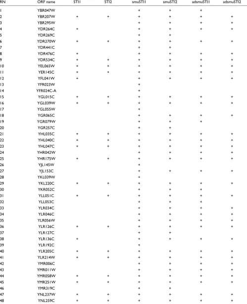
Table 2

Candidate differential expressed genes with different approaches

RN ORF name STI1 STI2 smuSTI1 smuSTI2 adsmuSTI1 adsmuSTI2

1 YBR047W + + +

2 YBR207W + + + + + +

3 YBR295W + + + +

4 YDR264C + + + + +

5 YDR269C + +

6 YDR270W + + + + + +

7 YDR441C + +

8 YDR476C + + + + +

9 YDR534C + + + + + +

10 YEL065W + + + + + +

11 YER145C + + + + + +

12 YFL041W + + + + +

13 YFR023W +

14 YFR024C-A +

15 YGL015C + + + + + +

16 YGL039W + + + + + +

17 YGL055W +

18 YGR065C + + + +

19 YGR079W + + +

20 YGR257C + +

21 YHL035C + + + + + +

22 YHL040C + + + + + +

23 YHL047C + + + + + +

24 YHR042W + + + +

25 YHR175W + + + + + +

26 YJL145W +

27 YJL153C + + + +

28 YKL039W +

29 YKL220C + + + + + +

30 YKR052C + + +

31 YLL051C + + + + + +

32 YLL053C + + +

33 YLR034C + + + +

34 YLR046C + + + +

35 YLR056W + + + +

36 YLR126C + + + + + +

37 YLR127C + +

38 YLR136C + + + + +

39 YLR192C +

40 YLR205C + + + + + +

41 YLR214W + + + + + +

42 YMR006C + + + +

43 YMR011W + + + +

44 YMR058W + + + + + +

45 YMR251W + + + + + +

46 YMR319C + +

47 YNL237W + + + + + +

(14)

49 YNR056C + + + + + +

50 YNR060W + + + + + +

51 YOL153C + + + + +

52 YOL158C + + + + + +

53 YOR334W + + + +

54 YOR381W + + + + + +

55 YOR382W + + + + + +

56 YOR383C + + + + + +

57 YOR384W + + + + + +

58 YPL171C +

59 YBR250W +

60 YDR423C +

61 YER028C +

62 YHR199C +

63 YIL169C +

64 YJL149W + + +

65 YOL101C + +

66 YOL164W + +

RN ORF name STI1 STI2 smuSTI1 smuSTI2 adsmuSTI1 adsmuSTI2

1 YBR054W + + + + +

2 YBR145W +

3 YBR147W + + + +

4 YCL030C + + + + +

5 YDL171C + + + + +

6 YDR035W + + +

7 YDR234W + +

8 YEL039C + + + +

9 YER001W +

10 YER156C + +

11 YER174C + + + + +

12 YFL014W + + + + +

13 YFR030W + + + + + +

14 YFR055W + + + +

15 YGL009C + + + + + +

16 YGL117W + + + + + +

17 YGR088W + + + +

18 YGR286C + + + + + +

19 YHL021C + + + + + +

20 YHL028W + + +

21 YHR018C + + + +

22 YHR029C +

23 YHR045W +

24 YIL111W + +

25 YJL048C + + +

26 YJL088W + +

27 YJL089W + +

28 YJL200C + + +

29 YJR016C +

[image:14.612.61.549.110.746.2]

30 YJR025C +

Table 2 (Continued)

(15)

comm

en

t

re

v

ie

w

s

re

ports

refer

e

d

re

sear

ch

de

p

o

si

te

d r

e

se

a

rch

interacti

o

ns

inf

o

rmation

candidates makes no assumptions about outlier distribution and dependency structure of the candidates. The mixture model of Sapir and Churchill [20] assumes that all candidates

have the same distribution D₀(D₀= D₁= ... = D_k, see

Meth-ods). Other approaches (for example, [17,19]) assume inde-pendence of channel intensities. The individual distributions are usually not known and could be different for each gene, since only replication allows estimation of the distributions. Multiple levels of dependence, such as co-regulated genes, are expected rather than unlikely in gene expression analysis. Since our model and analysis approach does not require such

assumptions, which are likely to be violated by the data, we would argue that our approach is more realistic and generally applicable.

Accommodating heteroscedasticity in outlier identification

We compensate for a source of reproducible systematic tech-nical error, heteroscedasticity, by using robust non-paramet-ric regression smoothers to quantify the differences in the variability of gene expression values as a function of spot intensity levels. STIs corrected for heteroscedasticity and

31 YJR109C + + +

32 YJR137C + + + + +

33 YKL062W + + +

34 YKL109W + + +

35 YKL141W + + +

36 YKL148C + + + +

37 YKL218C +

38 YKR066C + + +

39 YLL041C + + + + +

40 YLR220W + + +

41 YLR304C + + + + +

42 YMR021C + + + + + +

43 YMR022W + + +

44 YMR095C +

45 YMR096W + + +

46 YMR271C + +

47 YNL160W +

48 YOL058W + + +

49 YOL064C + +

50 YOR065W + + +

51 YOR195W + +

52 YOR230W +

53 YOR356W + + + +

54 YPL092W + + +

55 YPR123C + + +

56 YPR160W + +

57 YCR106W +

58 YGR052W +

59 YJR130C +

60 YOL119C +

61 YPL123C +

62 YPR167C +

Total 47 34 128 98 84 61

[image:15.612.57.558.107.547.2]

Candidates for differentially-expressed genes in the mac1 cDNA microarray experiment based on three different approaches: STI1 is ordinary STI at 99.98% and STI2, at 99.998%; smuSTI1 is supsmu-based STI at 99.98% and smuSTI2, at 99.998%; adsmuSTI1 is adjusted supsmu-based STI at 99.98% and adsmuSTI2, at 99.998%. The study monitored transcripts in a mac1 knockout and wild type S. cerevisiae. For the STIs, the above-mentioned captured portions of the respective normal distributions were covered with probability at least 99.99%.

Table 2 (Continued)

(16)

adjusted for Gaussian efficiency relative to the line of

equiva-lence (Cy5 = Cy3) serve as a probabilistic tool for identifying

outliers. Our approach uses robust scatter plot smoothing techniques to simultaneously diagnose and quantify the variance structure of the data and allow natural accommoda-tion of heteroscedasticity in the identificaaccommoda-tion of outliers. This

post hoc approach makes sense especially in view of the large sample size common in microarray experiments.

α

-Outlier-generating model can be extended to multiple slide studies

We can extend our adjusted smoothed STI approach to data-sets with multiple levels of replication. This provides a con-sistent method for experiments with and without replication. It is not clear how extant single-slide methods could be adapted for multiple-slide comparisons. Usually, two meth-ods, each with their own data models and assumptions - one for single-slide and a second for a multiple-slide based method, are used.

Transformations versus interpretation of microarray datasets

Our method is based on limited data transformations (for example, background subtraction, log-transformation and global channel normalization) designed to preserve the data distribution and account for heteroscedasticity. A variety of non-linear transformation methods can be used to remove heteroscedasticity, for example, variance-stabilizing monot-onic continuous non-linear transformations [21-23,44]. Equalizing residual variance in this manner does not guaran-tee that bivariate normality will be preserved for the majority of genes which are not differentially expressed. A model distribution assumption is especially important for statistical inference in the case of limited or no replication in the data. Non-linear transformation methods require preliminary research and computational experimentation with different types of transformations for each specific microarray dataset in order to make a choice between different transformations. Although transformation methods could represent a valuable

The use of smoothed absolute residuals to diagnose and quantify residual heteroscedasticity

Figure 11

[image:16.612.58.299.86.269.2] [image:16.612.57.298.498.671.2]

The use of smoothed absolute residuals to diagnose and quantify residual heteroscedasticity. 'Absolute residuals versus log2(Cy3)' scatter plot smoothed using supsmu and lowess and different values of the smoothing parameters bass and f, respectively. The figure illustrates the dependence of smoothing effect from magnitude of smoothing parameters. bass is control of the low frequency emphasis when using cross validation. The larger the value of bass (up to ten), the smoother the fit from automatic span selection [51,52,63]. f is fraction of the data used for smoothing at each log2(Cy3) point. The larger the f value, the smoother the fit [51,52,63].

The use of smoothed absolute residuals for sequential intensity intervals Figure 12

The use of smoothed absolute residuals for sequential intensity intervals. 'Absolute residuals versus log2(Cy3)' scatter plot based on supsmu and

lowess for 20 sequential intervals of equal size and using different values of smoothing parameters (see legend to Figure 11 for details). Data are shown with higher resolution than in Figure 13.

log₂(Cy3)

Absolute residuals

-15 -10 -5 0 5

cup5

bass = 0 bass = 2 bass = 4 f = 0.2 f = 0.4 f = 0.66

0 1 2 3 4 5 6

log₂(Cy3) medians for residual groups

Medians of absolute residuals

−4 −3 −2 −1 0 1 2 f = 0.66 f = 0.4 bass = 0 bass = 10

0.12 0.14 0.16 0.18 0.20 0.22 0.24

The use of smoothed absolute residuals for sequential intensity intervals Figure 13

The use of smoothed absolute residuals for sequential intensity intervals. 'Absolute residuals versus log2(Cy3)' scatter plot with supsmu and lowess smoothing based on 20 sequential intervals of equal size with shown values of smoothing parameters (see legend to Figure 11 for details). Scale is different from Figure 12.

log₂(

Cy

3)

Absolute residuals

−15 −10 −5 0 5

cup5

f = 0.2 (groups) bass = 10(groups)

(17)

comm

en

t

re

v

ie

w

s

re

ports

refer

e

d

re

sear

ch

de

p

o

si

te

d r

e

se

a

rch

interacti

o

ns

inf

o

rmation

approach to microarray data analysis, any complex non-lin-ear data transformation calls into question the validity of the transformations. Therefore, the application of these transformation methods requires trial and error followed by validation of each transformation for a particular experimen-tal dataset [44]. We suggest that our approach, which relies on interpretation of existing data distributions including any heteroscedasticity rather than application of methods to change distributions, provides a reasonable alternative to variance-stabilizing methods.

Multiple comparisons in microarray data analysis Typically, microarray data involve thousands of genes so clearly there is a problem of multiplicity of comparisons. Other model-based single-slide approaches do not consider this issue explicitly (see single-slide procedures described in [1,13,14,17,18]). First, we identify candidate outliers without

correction to obtain unadjusted p-values (Table 3). A p-value

is a probability to reject the null hypothesis when the null

hypothesis is true and represents a measure of statistical sig-nificance in terms of false positive rate. One way to obtain

adjusted p-values is to apply a Bonferroni correction based on

N (the sample size of the entire dataset) which may be too

conservative, so we examine two alternative corrections. In one alternative approach, we apply a multiplicity of

comparison correction based on an estimate of k (number of

non-regular observations) rather than the sample size of the entire dataset. This approach emphasizes stable outliers at

the expense of other possible outliers (that is, N-k) which are

inliers in the current single-slide experiment. Clearly, this

Bonferroni correction by k provides a much less conservative

result than the correction by N and we would argue more

reasonable correction to identify true outliers. Other robust

exploratory tools (see Methods) can be used to estimate k. In

a more sophisticated approach to address these issues, the q

-value is calculated from the ordered list of unadjusted p

-val-ues [45,46] (Figure 24). The q-value is the minimum false

dis-covery rate [47] for a particular feature from a list of all

[image:17.612.57.554.84.432.2]

Boxplots for residuals using ten sequential intervals of equal size Figure 14

Boxplots for residuals using ten sequential intervals of equal size. A box corresponds to the IQR (inter-quartile range), the mid point is a sample median, and whiskers are 3IQR limits. Outliers (non-regular observations) are points outside the whiskers. Abscissa is based on medians for ten intervals of approximately equal size (the total sample size is 6,068, the first nine sets were 606, the tenth set was 614).

−3.7 −2.6 −1.9 −1.5 −1.1 −0.7 −0.3 0.1 0.7 1.7 cup5

log₂(

Cy

3) medians for residual groups

log

2

(

Cy

5/

Cy

3)

−6

−4

(18)

features [45,46]. The false discovery rate is the proportion of true null hypotheses among all null hypotheses which were found to be significant - for example, a false discovery rate of 1% means that among all candidates for differential expres-sion found significant, 1% of these are true nulls on average [46].

Exploratory and confirmatory differential gene expression analysis

We suggest distinguishing explicitly between exploratory data analysis to identify candidates for differential gene expression and confirmatory analysis to identify differen-tially-expressed genes based on strict statistical inference. Exploratory differential gene expression analysis is appropriate for datasets with limited replication to identify the most likely candidates for differential expression. Clearly, additional independent experimental approaches or addi-tional replicates are needed to confirm the exploratory analysis and distinguish outliers by chance from systematic

outliers. Alternatively, confirmatory differential gene expres-sion analysis with multiple layers of experimental and techni-cal replication provides sound conclusions based solely on the microarray datasets. Nevertheless, exploratory microarray data analysis followed by independent confirmatory valida-tion studies (for example, quantitative RT-PCR) represents a practical and cost effective solution for expression studies.

Methods

Transcript profiling data

The transcript profiling datasets examined in this study are from a published study that employed cDNA microarrays to

compare gene expression in wild type S. cerevisiae and single

gene deletion mutants [18]. Hughes et al. monitored 6,295 S.

cerevisiae genes [18] in their study. For our analysis we used 6,068 of the 6,295 genes monitored. For each experiment, we used a Monte Carlo procedure to generate simulated datasets

of N = 6,068 data points drawn from an 'ideal' bivariate

[image:18.612.56.559.86.438.2]

Boxplots for residuals using 20 sequential intervals of equal size Figure 15

Boxplots for residuals using 20 sequential intervals of equal size. Details are the same as for Figure 14 but using 20 sequential intervals.

1 2 3 4 5 6 7 8 9 10 11 12 13 14 15 16 17 18 19 20 cup5

log₂(