On estimation of autoregressive conditional duration (ACD) models based on different error distributions

@

TI MALAYA

On

Estimation

of Autoregressive

Conditional

Duration

(ACD) Models Based

on

Different

Error Distributions

By:

D. Pathmanathan,

K.H. Ng

and

s.

Peiris

(Paper presented at the

International Statistics Conference 2010

held on 8-9 January 2010 in Colombo, Sri Lanka)

Sri Lankan Journal oj Applied Statistics, Vol.I 0, 2009,p.25J~269

On Estimation of Autoregressive

Conditional Duration (ACD)

Models Based on Different ErrorDistributions

D. PATHMANATHAN, K.H. NG" AND S. PErRIs ....

University of Malaya, Kuala Lumpur, Malaysia

ABSTRACT

Autoregressive Conditional Duration (A CD) models playa central role in modelling high frequency financial data. The Maximum Likelihood (ML) and Quasi Maximum Likelihood (QML) methods are widely used in parameter estimation. This paper considers a semi parametric approach based on the theory of Estimating Function (EF) in estimation of A CD models. We use a number of popular distributions with positive supports for errors and estimate the parameter(s) using the both EF and . ML approaches. A simulation study is conducted to compare the peiformance oj the EF and the corresponding ML estimates for ACD(1.1), ACD(l,2) and ACD(2,l) models. It is shown that the EF approach provides comparable estimates with the ML estimates using a shorter computation time. Finally, both methods are applied to ~odel a real financial data set and provide empirical evidence to support the use EF approach in practice.

Keywords: Conditional duration, Estimating function, High Frequency data,

Maximum likelihood

INTRODUCTION

In

many financial modelling problems, we face with the problem of analyzing high

frequency data. A class of high frequency data models are originally appeared

as

"fixed-interval" models, where all transactions are recorded as the fixed time intervals. However, one main drawback of these models is that they do not take into

account the irregular spacing of the data. As a result, we may lose some useful

information if the transactions cluster differently within a fixed interval. To avoid such loss of information, Engle and Russell (1998) had proposed the class of models

called the autoregressive conditional duration (ACD) models. This class of models

adapts the AR and GARCH theory to study the dynamic structure of the adjusted

durations and can be used to analyze transaction data with irregular time intervals .

---Let Xj be the adjusted duration such thatx,

=

t, - 1,_1, where 1j is the time of the ith

transacti on and let

(I)

where Fi-l is the information set available at the (i-1)th trade. The basic ACD model is defined as

(2)

where Cj is a sequence of independently and identically distributed (iid)

non-negative random variable's with density f(.)and E(ci)

=

1 and

s,

is independent of

F

i-l·

From Equation (2) it is clear that a vast set of ACD model specifications can be defined by allowing different distributions for

e,

and specifications of If!i .

A general class of ACD models generated from (2) is called

ACD (m,q),(m ~ 1,q ~0) and is given by

m q

III.

=

Ci)

+ "'"'

a .x. .

+ "'"'

b.,1//. .,

't'l L.... .I 1-.1 L.... /'1' 1-.1

i=i ;=1

(3)

r

where OJ> 0, aj,b.i > 0 and L(a; +b) <1, and r

=

max(m.q).

;=1

This paper focuses on the parameter estimation of ACD models based on a number of different distribution with positive support for Cj. Engle and Russel (1998) used

Likelihood (QML) methods. If the parameters in the model are not well-estimated, then the model may not be adequate for describing the behavior of the data. The accuracy of forecasts may also affect by a "poor" model.

In their paper, Peiris et al., (2007) suggested the use of the estimating function (EF) approach to estimate the parameters in ACD models. Peiris (2008) shows a simulation result of the estimation of ACD models using estimating functions.

Since the error distribution of the model is not known in practice, this paper extends the work of Peiris et.al.(2007) and focuses on the estimating parameters of ACD models based on various possible error distributions. We assess the performance of EF and ML methods and compare the bias and the standard errors in each case. We consider four popular different non-negative distribution for ci including the

Exponential, Rayleigh, Lognormal and Gamma to model ACD structures. Results show that both methods are comparable in estimating the parameters of the ACD models but the EF method proves to be faster and efficient than the ML for estimating the parameters when the distribution is unknown.

With that view in mind the following section reviews the parameter estimation problem based on the ML and EF approaches.

ESTIMATION

This section considers the ML and EF approaches to estimate the parameters of ACD models as well as the parameters of the corresponding error distributions.

The ML approach

Let iO

=

max(m,q) and xn

=

(xp".,xn)' for an ACD model, where n is the sample

size. The likelihood function for the durations is

n

L(xn

I

e,x

j)

=

TIf(xj

I

F;-I

,9)

where 9 denotes the vector of model parameters, Xio =(Xj,···,xio) and

;n

I'»;

19)

=

TIfe

Xi)·

i=1

As the sample size n increases, the impact of the marginal probability density function (pdf),

ts»;

19) on the likelihood function diminishes. Thus, the marginal density can be ignored resulting in the conditional likelihood function as below:

"

Lex"

19,

x;.)

=

TIfe

x; 1;;_1'9) .

;:::;0+1

(4)

For some selected distributions of

s.,

the likelihood functions are as shown below:

1. Standardized Exponential distribution: L(x

I

xio)

=TI

{_l e

-C~J}

/:::=10+1 Vlj

2. Standardized Rayleigh distribution: L(x

I

x

io)

=[1 {~( \

JeN~

II

'-'0 ~1 Ijf,

J

4. Standardized Gamma distribution: L(x

I

=:

=

TI

J[

K'·_

(!:i_JK-1

e-~:]_l

1

..

Now we consider the theory of estimating functions (EF) as an alternative semi-parameter approach for semi-parameter estimation.

The Estimating Function Approach

Let {Yb Y2, ...

J

be a discrete stochastic process. We are interested of fitting a

suitable model for a sample of size n from this process. Let

8

be a class of probability distributions

F

on

R

/1 and

B

=

B(F),

F

EGbe a vector of real

parameters.

Let hi be a real valued function of Yr, Y2,' .. , Yi and

B

such that

Ei-1,F[hi {Yl ,Y2," "Yi; f}(F)}]

=

0,

Ci

=

1,2,···,n;F E8)

and

EChihj)

=

0, (i:t: j), •

where Ei-1,F C·) denotes the expectation holding the first i-1' values

Yl,Y2,",Yi-l fixed and Ei-1,F(.)=Ei-1, EO,F(.)=EF(.)=E(.)Cunconditional

mean).

Estimating Functions

Any real valued function g(.) of the random variates Yl, Y2"", Y/1 and the parameter

B,

that can be used to estimate

B

is called an estimating function.

If gC:) satisfies regularity conditions (i) the first and the second derivatives of g(.), g' C·) and gilC.)exist, and Cii)E[g2 (.)] is non-zero

and

then g(.) is called a regular unbiased estimating function.

*

Among all regular unbiased estimating functions g , g is said to be optimum if

(5)

{E[[a

CY

1,Y2"",Yn;e)]

)}2

ae

!3=!3(F)

*

is minimized for all FEe at g

=

g .

Then, we estimate

e

by solving the optimum estimating equation

*

g (Yl, Y2 , ... , Yn ;e)

=

0 .

Main Results

We restrict initially to estimating functions g of the form

n

g

=

'2:

h;a;-l

1=1

where the functions h, are as defined before and a/-l is a function of the random variates Yl,Y2,",Y;-1 and the parameter

e

for all i=1,2,.. ·,n. We consider the class of linear estimating functions

L

generated by g. Note that g being linear in

hi' the class L corresponds to linear functions in Gauss-Markov set-up for linear models.

Clearly,

E(g)

=

0,

gEL.

Now we state the following theorem due to Godarnbe(l985):

Theorem

*

In

the class L of estimating functions g , the function g minimizing (5) is given by

*

n

*

g

=

Ih;a;_l ,

i==1

where

[OhiJ

E.

1-*

/-

of}

Qi-l

=

2'

£,-l[h, ]

Notes:

*

1. The functiong is called the optimum estimating function.

2. Based on Godambe (1985), an optimal estimate of f} can be obtained by

*

solving the equation(s) g

=

O.

See Thavaneswaran and Abraham (1988) and Grahramani and Thavaneswaran (2009) for theory and various applications of estimating functions.

Estimation of ACD (m,q) Using the EF Approach

Consider the ACD (m,q) model given by Equations (2) and (3). It is clear that the conditional distribution

where' [2i_1 is the information set available at time i-I and

u~

is the variance of

e.,

Let hi

=

Ifi - Xi' It is obvious that hi is an unbiased estimating function. Now, a

linear unbiased estimating function is constructed such that

11

0== '\' h.a~

o ~ I I'

,;1

Ol/f,

where a~==

a,e

and

e

is a parameter.

, 1jI,~V

Solving the following system of Equation (6) for

e

and the optimal set of estimates can be obtained:

(6)

The following derivatives under the conditions of i-th order stationarity can be used:

•

•

aw, _

~

b Ol/f'-i

---V!,-,+

~

j--obi ,;1.j='. obj

where k and 1 are respectively the subscripts of the parameter of interest for a and

b.

•

Itis easy to see that for ACD( 1,J ) model, we have

(7)

where

s

is the variance of £, .

For example,

a) s ==.2 for standardized Exponential distribution

b)

s

=

i

for standardized Rayleigh distribution

J[

c) s

=

ea2 for standardized Lognormal distribution

d)

s

=

K + 1 for standardized Gamma distribution K

SIMULATION

This section considers a large scale simulation study in order to compare the performances of the MLE and EF approaches for an ACD(l,l) model based on a number of standardised distributions as mentioned above in (a) to (e). Let

e

be an estimator of parameter 8. Suppose that we simulate a series of length n and estimate respective parameters. Repeat these simulation and estimation steps N

times and calculate the following:

-

1

N

i) Mean,

e

=-

~e

Nt;j'

ii) Estimated Bias = 8 -8

.. lati E' dB' (0/)

(I

Estimated Bias

I)

ill) Absolute Re atrve stimate las /0

=

8 . .xl 00%

iv) Estimated Standard Deviation (S.D) =

-1-f(e

_0)2

N-l ;=J

v) Mean Squared Error, MSE(e) =

Elce -

8)2

J

~ 2

=

Var(8)

+

(bias)

. . . Estimated SD of EF

VI) Relative Efficiency

=

---Estimated SD of ML

For the Exponential ACD (EACD) case EACD(l, 1), EACD(2, J), EACD(l, 2) and EACD(2, 2) have been studied and the corresponding estimating results have been reported in Tables 1 to 4. It seems that the results obtained using the ML and EF methods are comparable. However, the EF method provides smaller estimated standard error in estimating the parameters

b

1 and

b'2

for both EACDC1, 2) (in Table

l.:

3) and EACD(2, 2) (in Table 4) models. Although the absolute relative bias, the. means of

b

l and

b

2 seem to be slightly better in ML estimates than the EF method,

the computation time is relatively smaller in the EF approach. When the Mean Squared Error (MSE) is scrutinized for the case involving the EACD(1, 2) model,

e

)

.

.

the results for

b,

and b:. appear to be comparable. The MSE for OJ is slightly larger

.

.

when EF is applied. The MSE computed for W , b, and h:. are smaller when the EF approach is utilized in estimating the parameters of the EACD(2, 2) model.

A similar conclusion can be drawn for Lognormal ACD (1,1) model, Rayleigh ACD (1, 1) model and Gamma ACD model(GACD(l, 1)) (Refer to Tables 5 to 7) the estimates of the parameters are somewhat comparable for both EF and ML methods. In general, the EF method's computation time is 5 times faster compared to the ML method.

Table 1: Estimated Results for Simulated Exponential ACD (1, 1) Series with 500

observations ((j)

=

0.20,

a

l

=

0.30, b. =0.60 and fill =0.50).

to a) hI

ML

EF

ML

EF

ML EF

Mean 0.2198 0.2205 0.2977 0.2949 0.5893 0.5905

Estimated Bias 0.0198 0.0205 -0.0023 -0.0051 -0.0107 -0.0095

Abs. Rel. Est. Bias 9.90% 10.25% 0.77% l.70% 1.78% 1.58%

Estimated S.D. 0.0715 0.0695 0.0527 0.0521 0.0686 0.0689

MSE 0.0055 0.0053 0.0028 0.0027 0.0048 0.0048

Relative Efficiency

I

1.0000

I

0.9720 1.0000 0.9886 1.0000 1.0044

Table 2: Estimated Results for Simulated Exponential ACD (2, 1) Series with 500 observations

t

to :;:0.10, aJ =0.20,a1 =0.30,bJ =OAO, Ifl =OAO and If 1=0.60).

co aJ G2 _bJ

ML EF ML EF ML EF ML EF

Mean 0.1082 0.1082 0.1961 0.1959 0.2953 0.2957 0.3928 0.3924

Estimated

0.0082 0.0082 -0.0039 -0.0041 -0.0047 -0.0043 -0.0072 -0.0076 Bias

Abs. Rel.

8.20% 8.20% 1.95% 2.05% 1.57% 1.43% 1.80% 1.90% Est. Bias

Estimated

0.0322 0.0321 0.0564 0.0563 0.0815 0.0817 0.0917 0.0913 S.D.

MSE 0.0011 0.0011 0.0032 0.0032 0.0067 0.0067 0.0085 0.0084

Relative

1.0000 0.9969 1.0000 0.9982 1.0000 1.0025 1.0000 0.9956 Efficiency

Table 3: Estimated Results for Simulated Exponential ACD (1, 2) Series with 500

observations (())=0.10,G] =0.20,bl

=

0.30,b2 =0.40,If] =0.40 and 1f2 =0.60)

co

_I

G]

₆

₁

b1

ML EF

I

ML EF ML EF ML EF

Mean 0.1249 0.1236 0.1924 0.1827 0.3516 0.4238 0.3281 0.2652

Estimated

0.0249 0.0236 _0.00761-0.0173 0.0516 _{0.1238 -0.0719}

-0.1348 Bias

Abs. Rel.

24.90% 23.60% 3.80% 8.65% 17.20% _{41.27% 17.98%}

33.70% Est. Bias

Estimated

0.0817 0.1107 0.0552 0.0551 0.3245 _{0.3101 0.2870}

0.2586 S.D.

MSE 0.0073 0.0128 0.0031 0.0033 0.1080 0.1115 0.0875 0.0850

Relative

1.0000 1.3550 1.0000 0.9982 1.0000 _{0.9556 1.0000}

0.9010 Efficiency

Table 4: Estimated Results for Simulated Exponential ACD (2, 2) Series with 500 observations ((v=OAO,(l1 =O.lO,a:, =0.20,bl =O.20,b] =OAO,1f1 =0.50 and

It.']

=

0.50)

OJ (ll

u]

bl b,

ML EF ML EF ML EF ML EF ML EF

t\~m 0.4428 0.4192 0.OY33 0.0967 0.180710.1641 0.3161 0.3870 0.2938 0.2425

Esti "luted

0.0428 0.0192

-

- - -00359 0.1161 -0.1062

BiOS 0.0067 0.0033 0.0193 0.1870 -01575

Abs. ReI.

10.70% 4.80% 6.70% 3.30% 9.65% 17.95% 58.05% 93.50% 26.55% 39.38% Est. Bas

Estirna ed

0.2064 0.1849 0.0524 0.0515 0.0831 0.0824 OA155 0.3593 0.3308 0.2817 S.D.

MSE 0.0444 0.0346 0.0028 0.0027 0.0073 0.0081 0.1861 0.1641 0.1207 0.1042

Relative.

1.0000 0.8958 1.0000 0.9828 1.0000 0.9916 1.0000 0.8647 1.0000 . 0.8516 . Efficiency

Table 5: Estimated Results for Simulated Rayleigh ACD (1, 1) Series with 500

observations (OJ = 0.05,a =0.30,bl = 0.60 and Ifl = 0.50)

OJ al bl

ML EF ML EF ML EF

Mean 0.0559 0.0555 0.2986 0.2966 0.5877 0.5912

Estimated Bias 0.0059 0.0055 -0.0014 -0.0034 -0.0123 -0.0088

Abs. Rel. Est. Bias 11.80% 11.00% 0.47% 1.13% 2.05% 1.47%

Estimated S.D. 0.0169 0.0171 0.0386 0.0403 0.0577 0.0589

MSE 0.0003 0.0003 0.0015 0.0016 0.0035 ₁ 0.0035

Relative Efficiency 1.0000

I

1.0118 1.0000 1.0440 1.0000 1.0208

Table 6: Estimated Results for Simulated Lognormal ACD (1, 1) Series with 500 observations (UJ

=

O.lO,a =0.20,bl

=

0.70,0"

=

1.50 and lfIl

=

0.50)

UJ QI _b

l (J

ML EF ML EF _{ML EF ML EF}

Mean 0.1151 0.1160 0.1985 0.1974 0.6855 0.6857 0.4983 0.4913

Estimated

I

0.0151 0.0160 -0.0015 -0.0026 -0.0145 -0.0143 -0.0017 -0.0087 . Bias

Abs. ReI. Est.

15.10% 16.00% 0.75% 1.30% 2.07% 2.04% 0.34% 1.74% Bias

Estimated

0.0401 0.0442 0.0372 0.0400 0.0637 0.0690 0.0157 0.0267 S.D.

MSE 0.0018 0.0022 0.0014 0.0016 0.0043 0.0050 0.0002 0.0008

Relative

1.0000 1.1022 1.0000 1.0753 l.0000 1.0832 1.0000 1.7006 Efficiency

Table 7: Estimated Results for Simulated Gamma ACD (1, 1) Series with 500

observations (UJ

=

0.05,

a.

=

0.20,b, =0.70,K

=

1.50 and IfII

=

0.50)

UJ aJ h_J

K

ML EF ML EF ML EF ML EF

Mean 0.0584 0.0590 0.2004 0.2010 0.6820 0.6797 1.5169 1.6055

Estimated

_-

-0.0169

0.0084 0.0090 0.0004 0.0010 _0.1055

Bias _{0.0180 0.0203}

Abs. Rel.

16.80% 18.00% 0.20% 0.50% 2.57% 2.90% 1.13% 7.03%

Est. Bias

Estimated

0.0230 0.0238 0.0420 0.0419 0.0721 0.0736 0.0881 0.2518

S.D.

MSE 0.0006 0.0006 0.0018 0.0018 0.0055 0.0058 0.0080 0.0745

Relative

1.0000 1.0348 1.0000 0.9976 1.0000 1.0208 1.0000 2.8581

Efficiency

APPLICATION OF ACD MODELS IN FINANCIAL DATA

As an analogy of duration models in financial data set, the transaction durations of IBM stock on five consecutive trading days from November 1 to November 7, 1990 was considered. This data was obtained from (Tsay,2002). We have 3534 observations where the positive transaction durations were focused on. In a nutshell, we employ 3534 positive adjusted durations. Figures 1 to 3 are respectively the series, the histogram of the series and the autocorrelation (ACF) of the series. Based on Figure 3, there exist some serial correlations in the adjusted durations.

500 1000 1500 2000 2500 3000 3500

secuence

Figure 1:Time plots of durations for

IBM

stock traded in the first five trading days

of November 1990: the adjusted series.

1000

3000

2000

1D 20 30 '0 '0

Adjusted series

c

-..

.;

~

'"

u,

o

<

.

'"

" 0

0 jill 11 I , _I

'"

10

I II·

20 30

[image:17.450.7.444.18.566.2]

Lag

Figure 3: ACF of the adjusted series

Based on the above analysis, we have fitted the ACD(l, 1) model from the distributions proposed earlier using both ML and EF methods for each of the distribution. Inall cases we have use If/]

=

1.0 as the initial value.

The ACD(1, 1) model is represented by:

and

where

{cj}

is a sequence of independent and identical non-negative random variables with density f(.) and E(E:j)

=

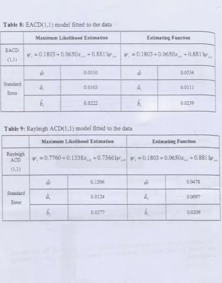
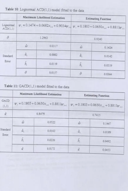
1.

The corresponding results are shown in Tables 8 to 11. As before, for this data set, the results for the parameter estimates are comparable except for the Rayleigh distribution.

[image:18.450.7.446.19.580.2]

Table 8:EACD(l, 1) model fitted to the data

--Maximum Likelihood Estimation Estimating Function

EACD

If, =:0.1803

+

0.0650x'_1

+

0.88111,11,_1 lfI, =:0.1803

+

0.0650x'_1 + 0.88111fH

(1,1)

-to 0.0510 _co 0.0534

Standard

0.0103 0.0111

al al

Error

bl 0.0222 hi 0.0239

Table 9:Rayleigh ACD( 1,1) model fitted to the data

Maximum Likelihood Estimation Estimating Function

Rayleigh

lfI, =:0.7760

+

O.1338xi-J

+

O.73661V/'_1 lfIi

=

0.1803

+

0.0650xi_1 +O.8811Ifi_1 ACD

(1,1)

co 0.1206 U) 0.0478

Standard

0.0124

al al 0.0097

Error

b[

0.0277

b

l 0.0209

[image:19.450.5.441.16.665.2]

Table 10:

Lognormal

ACD(l,

1) model fitted to the data

Maximum Likelihood Estimation _{Estimating Function}

Lognormal _{If, =0.1474+0.0682x'_1 +0.90341f,_}

If, =0.1803+0.0650x'_1 +0.88111f1'_1

ACD(l,l)

(J" _1.2963

0.9240

0) 0.0317

I

co 0.1424

al _{0.0082 a}

l _0.0142

Standard

Error

bl 0.0119 _b

l _0.0519

(J" _{. 0.0157}

(J" _0.0364

Table

11:

GACD(l,l)

model fitted to the data

Maximum Likelihood Estimation

Estimating Function

GACD

If, =0.1803+0.0650x'_1 +0.8-8111,ll'_1 _{1,lI, =0.1803+0.0650x'_1 +0.88111,ll'_1}

(1,1)

K

I

0.8479 0.7415

co 0.0522 ₀₎

0.1447

Standard _al

I

0.0102 al _0.0189

Error

b. 0.0226 _{bl 0.0492}

K 0.0172 _{K 0.0453}

CONCLUDING REMARKS

This paper reviews the theory of ACD models and two estimations methods based on the MLE and EF approaches. Based on a simulation study we have noticed that both methods are comparable but the EF method is computationally efficient.

Although the EF approach is easy to apply in practice, the ML estimates are better than the EF estimates when the true distribution is known. In practice, the EF approach gives reliable estimates as the true distribution is unknown. Using the recent result of Grahramani and Thavaneswaran (2009) it can be shown that the EF approach is superior and this will be further investigated in a future paper.

ACKNOWLEDGEMENT

Authors thank three anonymous referees and the editor for their valuable comments and useful suggestions to improve the readability of this paper.

REFERENCES

Allen, D., F. Chan, M. McAleer and M.S. Peiris (2008). Finite sample properties of QMLE for the Log-ACD model: Application to Australian stocks. Journal of Econometrics, 147: 163-185.

Allen, D., D. Zdravetz and M.S. Peiris (2009). Comparison of alternative ACD models via density and interval forecasts: Evidence from the Australian

Stock Market. Mathematics and Computers in Simulation, 79(8): 2535-2555. Engle R.F. and lR. Russell (1998). Autoregressive conditional duration: A new

model for irregularly spaced transaction data. Econometrica, 66(5): 1127-1162.

Godambe, V.P. (1985). The foundations of finite sample estimation in Stochastic processes. Biometrika, 72(2): 419-428.

Grahramani, M. and A. Thavaneswaran (2009). Combining estimating functions for volatility. Journal of Statistical Planning and Inference, 139(4): 1449-1461. Pacurar, M. (2008). Autoregressive conditional duration models in finance: A survey

of the theoretical and empirical literature. Journal of Economic Surveys,

22(4): 711-751.

Peiris, M.S., D. Allen and K.H. Ng (2008). Estimation of ACD models using estimating functions: A simulation study. Modelling and Managing Ultra High Frequency Data: An International Conference (MMUHFDIC 2008),

13-141h Feb 2008, Perth, Australia.

Peiris, M.S., K.B. Ng and LB. Mohamed (2007). A review of recent developments of financial time series: ACD modelling using the estimating function approach. Sri Lankan Journal

0/Applied Statistics,

8: 1-17

Thavaneswaran and Abraham (1988). Estimation of nonlinear time series models using estimating equations. Journal a/Time Series Analysis, 9: 99-108. Tsay, R.S. (2002). Analysis a/Financial Time Series. John Wiley & Inc., New York.