E c olo gi c al a n d e v ol u tio n a r y
c o n s e q u e n c e s of a l t e r n a tiv e s e
x-c h a n g e p a t h w a y s i n fis h
B e n v e n u t o , C, C o s ci a , I, C h o p e l e t , J, S a l a-Boz a n o , M a n d M a ri a n i, S
h t t p :// dx. d oi.o r g / 1 0 . 1 0 3 8 / s 4 1 5 9 8-0 1 7-0 9 2 9 8-8
T i t l e
E c olo gi c al a n d e v ol u tio n a r y c o n s e q u e n c e s of a l t e r n a tiv e
s ex-c h a n g e p a t h w a y s in fis h
A u t h o r s
B e n v e n u t o , C, C o s ci a , I, C h o p el e t, J, S al a-Boz a n o , M a n d
M a r i a n i, S
Typ e
Ar ticl e
U RL
T hi s v e r si o n is a v ail a bl e a t :
h t t p :// u sir. s alfo r d . a c . u k /i d/ e p ri n t/ 4 3 2 9 5 /
P u b l i s h e d D a t e
2 0 1 7
U S IR is a d i gi t al c oll e c ti o n of t h e r e s e a r c h o u t p u t of t h e U n iv e r si ty of S alfo r d .
W h e r e c o p y ri g h t p e r m i t s , f ull t e x t m a t e r i al h el d i n t h e r e p o si t o r y is m a d e
f r e ely a v ail a bl e o nli n e a n d c a n b e r e a d , d o w nl o a d e d a n d c o pi e d fo r n o
n-c o m m e r n-ci al p r iv a t e s t u d y o r r e s e a r n-c h p u r p o s e s . Pl e a s e n-c h e n-c k t h e m a n u s n-c ri p t
fo r a n y f u r t h e r c o p y ri g h t r e s t r i c ti o n s .
Ecological and evolutionary
consequences of alternative
sex-change pathways in fish
C. Benvenuto
1, I. Coscia
1, J. Chopelet
2, M. Sala-Bozano
2& S. Mariani
1Sequentially hermaphroditic fish change sex from male to female (protandry) or vice versa (protogyny), increasing their fitness by becoming highly fecund females or large dominant males, respectively. These life-history strategies present different social organizations and reproductive modes, from near-random mating in protandry, to aggregate- and harem-spawning in protogyny. Using a combination of theoretical and molecular approaches, we compared variance in reproductive success (Vk*) and effective
population sizes (Ne) in several species of sex-changing fish. We observed that, regardless of the
direction of sex change, individuals conform to the same overall strategy, producing more offspring and exhibiting greater Vk* in the second sex. However, protogynous species show greater Vk*, especially
pronounced in haremic species, resulting in an overall reduction of Ne compared to protandrous species.
Collectively and independently, our results demonstrate that the direction of sex change is a pivotal
variable in predicting demographic changes and resilience in sex-changing fish, many of which sustain highly valued and vulnerable fisheries worldwide.
Unique among vertebrates1, sex-changing fish develop and reproduce as males first and then grow into highly
fecund females (protandry), or reproduce initially as females to later change into large dominant males (pro-togyny). Sequential hermaphroditism has intrigued evolutionary biologists for decades and a great amount of information has been gathered on sex determination, sex differentiation and the plasticity of sex change in fishes2–5. The main theoretical model proposed to explain its adaptive value, the size advantage model6–8, predicts
that sex change should occur when the reproductive success of an individual depends on its size, but more so for one sex than the other. In this scenario, protandry is favoured over fixed separate sexes (gonochorism) when larger females have higher reproductive value than smaller ones (they can produce more eggs), while protogyny is favoured in situations where size allows dominant males to control the reproductive access to females.
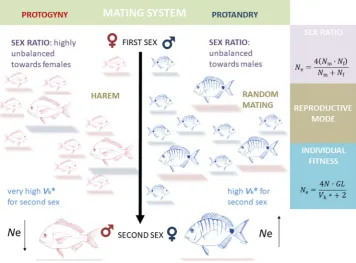
At the population level, we can expect that the variance in individual lifetime reproductive success (Vk*) will
influence the demographic trajectory of a population (Fig. 1). Strangely, sex-changing populations have seldom been investigated from a population genetic perspective. In those circumstances the focus has been only on one sex-changing mode, mainly protogyny9, 10 or on the comparison between gonochoristic and sex-changing
species11, 12. Yet, among sequential hermaphrodites, protandry and protogyny stand as two remarkably different
life-history strategies as they are shaped by different social systems and reproductive modes3, 5, 13. In protandrous
species, populations are composed of many small males and fewer large, highly fecund females. The reproductive mode is often monogamy or near-random mating2, 6. Protogyny, on the other hand, occurs when there is high
potential for polygyny and results in strong social structures dominated by large males6, 8, in some cases
antag-onised by sneakers. Males are territorial and control harems of females or, in group-spawners, larger males are expected to be the most successful. In either case, in protogyny there is a strong sexual selection on males.
Mating system and reproductive mode variations are predicted to influence Vk*14 (Fig. 1). In particular, Vk*
should be greater in protogyny than in protandry, as large males can monopolize multiple females and small females will tend to choose the larger males, increasing the reproductive success of a small number of larger males.
As a result of such changes over an individual’s lifetime, sequentially hermaphroditic species typically exhibit sex ratios that depart from the balanced ≈ 0.5 observed in gonochoristic species, and are generally skewed towards the ‘first sex’. Such a bias is more pronounced in protogynous species than protandrous ones15. Variance
1Ecosystems and Environment Research Centre, School of Environment & Life Sciences, University of Salford,
Salford, M5 4WT, UK. 2School of Biology and Environmental Science, UCD University College Dublin, Belfield, Dublin,
Ireland. Correspondence and requests for materials should be addressed to C.B. (email: [email protected])
Received: 4 May 2017 Accepted: 25 July 2017 Published: xx xx xxxx
www.nature.com/scientificreports/
in reproductive success and skewed sex ratios are the two most powerful forces that shape a parameter of crucial significance in population genetics, ecology and conservation: the effective population size (Ne), which offers a
view of the intensity of genetic drift and the changes in genetic variability in a population and its potential for persistence and resilience16, 17. Wright18 was the first to realize that the “effective population number” should
refer only to the “breeding population and not to the total number of individuals of all ages”; indeed, the effective population number in natural populations is generally smaller than the census size of the same population, some-times by one or more orders of magnitude.
The direct influence of skewed sex ratio applies mainly to gonochoristic species. In sequential hermaphrodites, the sex ratio is dynamic and many individuals contribute to the coming generations as both sexes (even though not all individuals change sex). Biased sex ratios though reinforce reproductive skew, and higher Vk* values
indi-cate that female-first sex-changers should have lower Ne than male-first sex-changers (Fig. 1). Thus, the direction
of sex change is expected to have an influence on Ne and, consequently, on population structure.
Calculating Ne is extremely difficult because it requires a specific knowledge of the demographic and
eco-logical parameters of the natural population under study. As mentioned, Ne can be influenced by a multitude of
factors, including fecundity, birth rate, natural mortality, migration, breeding sex ratio, variance in family size, age-structure, spatial and temporal distributions and reproductive mode19. For this reason, direct demographic
methods of calculating Ne are often replaced by indirect genetic methods20.
Here, we used a combination of theoretical modelling and molecular genetics to compare the effective popu-lation size in several species of protandrous and protogynous fish. A life-history model21 was employed to
esti-mate Ne, Vk*, the effective number of breeders per year (Nb), as well as the annual mean number of offspring ( ) k¯
and Vk and Nb for each sex in two sets of protandrous and protogynous species. At the same time, molecular
markers were used to produce empirical Nˆe estimates for a similar set of protandrous and protogynous species. The combination of these two approaches largely confirms the main expectation of lower Ne estimates for
pro-togynous than for protandrous species, and collectively unveils previously unrecognised patterns and trends that are of great relevance to the management of marine living resources.
Results
Life history modelling.
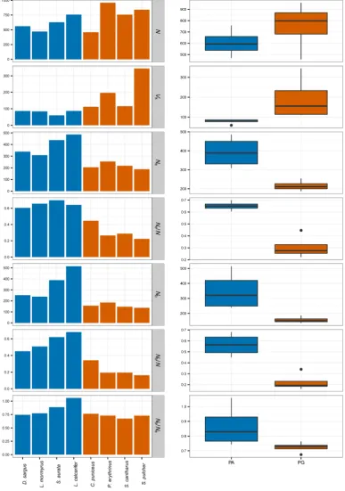
A range or realistic life-table scenarios were produced, utilizing data from literature on eight species, four protandrous (PA) and four protogynous (PG; Table 1), to estimate21 multiple keypopula-tion parameters (Table 2). As predicted, protogynous species overall showed significantly lower Ne (mean ± sd:
PG = 215.73 ± 28.06; PA = 392.70 ± 83.28; t = 4.03, df = 6, p = 0.006; Fig. 2) and higher lifetime Vk* (mean ± sd:
PG = 191.61 ± 108.59; PA = 78.90 ± 12.88; W = 0, p = 0.029; Fig. 2) than protandrous species, in the face of a stable total adult N (adult census size) that did not differ significantly between the two groups (mean ± sd: Figure 1. Interplay among individual fitness, life-history traits and population dynamics. Multiple factors affect effective population size (Ne), including many driven by the mating context of the population. The exemplified
protogynous species is drawn in red and the protandrous one in blue; shadows indicate the sex of individuals at any point during their lives (red for females; blue for males). In the equations: Nm= number of adult
males; Nf= number of adult females; N= total number of adults in the population; GL= generation length;
[image:3.595.157.514.47.310.2]PG = 753.00 ± 213.41; PA = 603.50 ± 120.87; t =−1.22, df = 6, p = 0.280; Fig. 2). Similarly, no significant dif-ference was detected in generation length (mean ± sd: PG = 10.24 ± 5.02; PA = 7.88 ± 1.94; t =−0.87, df = 6, p = 0.416). Indeed, the linear model returned protogyny (t =−7.280; p < 0.001) as the main factor reducing the size effective ratio Ne/N, which allows to control for the variance in population abundance estimates (N).
As all the species under study are iteroparous, Nb (effective number of breeders per breeding cycle) was
also calculated and found to be significantly lower in protogynous than in protandrous species (mean ± sd: PG = 155.98 ± 20.91; PA = 348.20 ± 129.91; W = 16, p = 0.0286; Fig. 2). The linear model returned protogyny (t =−6.179, p = 0.003) as the main factor reducing Nb/N (again, to control for the variance in population
abun-dance estimates, N), with maximum length as a covariate, which significantly increased this size effective ratio (t = 2.954, p = 0.042).
The analysis of the Nb/Ne ratio revealed no influence of the mating system (t =−2.074; p = 0.093), but a
sig-nificant effect of maximum length (t = 4.886; p = 0.004). The male-first sex-changer L. calcarifer showed a ratio larger than 1 (Nb/Ne= 1.059), meaning that in this species the number of breeders per year is actually higher than
the overall effective population size (Fig. 2).
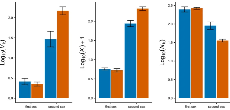
It was also possible to analyse k¯, and annual Vk and Nb for each sex. Graphically (Fig. 3) it is easy to visualize
the reproductive strategy for an individual when it reproduces as a different sex during its lifetime, changing from the first sex (male in protandry and female in protogyny) to the second sex (female in protandry and male in protogyny). Individuals belonging to protandrous species have higher annual k¯ (mean ± sd: ♀ = 7.17 ± 2.26; ♂= 0.55 ± 0.06; = 5.06, df = 6, p = 0.002) and Vk (♀= 22.70 ± 14.80; ♂= 2.24 ± 0.75; t = 5.06, df = 6, p = 0.002)
when they are older and larger (second sex, female, Fig. 3a). For this latter stage of life (the female phase), in the population there are fewer breeders per year than for the male phase (Nb♀= 124.20 ± 52.39; Nb♂= 299.00 ± 87.71;
t =−3.561, df = 6, p = 0.012). A mirrored situation applies to protogynous species, and in this case the magnitude is even stronger (Fig. 3b): larger males second sex) have much higher annual k¯ (♂= 17.82 ± 4.04; ♀= 0.51 ± 0.09;
Species Family Reproductive mode AgeMax Linf t0 K tm α β
Protandry
Diplodus sargus Sparidae Broadcast spawners 1263 45.90 −0.890 0.171 3 0.011 5.1064
Lithognathus mormyrus Sparidae Broadcast spawners 1165 38.4466 −1.48366 0.20066 3 0.010† 5.10†
Sparus aurata Sparidae Broadcast spawners 1267 59.7667 −1.71167 0.15367 2 0.010† 5.10†
Lates calcarifer Latidae Broadcast spawners 23[32]68 143.00 −0.860 0.130 4 27.00069 2.8969
Protogyny
Chrysoblephus puniceus Sparidae Haremic 1012 44.0070 −0.810 0.180 2 10.253* 2.6071
Pagellus erythrinus Sparidae Group spawners 2131 41.7872 −1.210 0.130 3 0.030‡ 5.49‡
Spondyliosoma cantharus Sparidae Haremic and nest guarders 1073 47.70 −0.830 0.180 2 0.04074* 4.6074*
Semicossyphus pulcher Labridae Haremic and territorial 2947 55.77 −0.710 0.126 4 0.00189 5.4975
Table 1. Parameters utilized to construct life history tables. AgeMax: maximum age (in years; in square brackets maximum age recorded for few individuals, not used in the model); Linf: asymptotic length (in cm);
K: growth coefficient; t0: theoretical age at length = 0; tm: age at first maturity; α: constant in the fecundity
relationship (adjusted to standard length); β: exponent in the fecundity relationship. Values are obtained from FishBase49 unless specified. *Values calculated from available data for Spondyliosoma cantharus74; †data
obtained for D. sargus; ‡extrapolated values from fecundity.
Species Total N N GL Vk* Ne Ne/N Nb Nb/N Nb/Ne tc ♀ k ♀ Vk ♀ Nb ♂ k ♂ Vk ♂ Nb
Protandry
Diplodus sargus 1875 560 7.449 85.960 338.7 0.605 251.9 0.450 0.744 6 7.650 32.510 91.7 0.573 3.089 201.3
Lithognathus
mormyrus 1767 470 6.591 83.526 308.2 0.656 238.2 0.507 0.773 6 9.942 37.910 78.3 0.600 2.651 248.7
Sparus aurata 1957 627 6.751 59.668 437.9 0.698 388.2 0.619 0.887 6 6.592 13.110 131.8 0.554 1.751 368.0
Lates calcarifer 2356 757 10.745 86.435 486.0 0.642 514.5 0.680 1.059 8 4.508 7.282 195.0 0.469 1.487 378.0
Protogyny
Chrysoblephus
puniceus 1755 458 5.810 111.782 204.2 0.446 155.9 0.340 0.763 5 0.588 1.844 366.9 18.170 18.170 43.6
Pagellus
erythrinus 2326 958 12.564 196.089 253.7 0.265 185.0 0.193 0.729 9 0.443 1.733 297.7 14.610 67.680 54.8
Spondyliosoma
cantharus 1756 756 6.352 114.935 217.3 0.287 146.5 0.194 0.674 5 0.592 2.435 269.5 15.120 143.000 42.4
Semicossyphus
pulcher 2455 840 16.219 343.616 187.7 0.223 136.5 0.163 0.727 13 0.415 1.619 301.0 23.410 83.32.0 38.5
Table 2. Estimates from AgeNe and used value of age at sex change (tc) for each species. Total N: estimated
number of individuals in the population; N: estimated number of adult individuals (adult census size); GL: estimated generation length; Vk*: lifetime variance in reproductive success; Ne: effective population size; Nb:
www.nature.com/scientificreports/
Welch t-test t =−24.892, df = 5.87, p < 0.0001), higher Vk (♂= 78.03 ± 51.43; ♀= 1.91 ± 0.36; W = 0, p = 0.029),
and lower Nb than smaller females, the first sex (♂= 44.83 ± 7.00; ♀= 308.78 ± 41.25; W = 16, p = 0.029). The
even greater mismatch between the number of breeders for the two sexes reflects nicely the description of haremic species, where few males monopolize the majority of females.
Figure 2. Graphical representation of some key population parameter estimates (obtained with AgeNe) by individual species (panel a) and mating system (panel b); protandry in blue vs. protogyny in red. N: estimated number of individuals in the population (census size); Vk*: lifetime variance in reproductive success; Ne:
effective population size; Nb: effective number of breeders per year. Key ratios (Ne/N, Nb/N and Nb/Ne) are also
[image:5.595.155.543.49.601.2]In general, the trend is similar between protandry and protogyny: the second sex has always higher k¯ and Vk
(which confirms the individual advantage of a change of sex in both systems) and lower Nb than the first sex
(Fig. 3). When comparing the reproductive success of first and second sex across the two systems, it is interesting to see a significant interaction (mating system [PA, PG] crossed with sequential sex [first, second]: t = 26.06; P < 0.0001; Fig. 4): the second sex is comparatively more successful in protogyny, whereas the first sex is slightly more successful in protandry. Protogynous male breeders (second sex in red in Fig. 4) are more successful (but less numerous) than protandrous females (second sex in blue in Fig. 4) but protogynous females (first sex in red in Fig. 4) are not more successful than protandrous males (first sex in blue in Fig. 4), even though at this stage the fitness difference between the first and second sex is not as large as it will become later in life, after sex change.
Genetic evidence.
We had generated genotypic data from five sparid species: three protandrous, Diplodus sargus, Lithognathus mormyrus22 and Sparus aurata23, and two protogynous, Chrysoblephus puniceus12 and Pagellus erythrinus24. Furthermore, two more protogynous species, Cephalopholis fulva and Epinephelus guttatus,were included in the analyses, based on datasets made available by Portnoy and colleagues9. No significant signals
of large allele drop out, scoring error were detected across each species. Only C. puniceus had one marker (SL35) that had a strong probability for null alleles, and was hence removed from the statistical analysis. Average observed (Ho) and expected (He) heterozygosities were respectively 0.756 and 0.823 for D. sargus; 0.844 and 0.836
for L. mormyrus; 0.768 and 0.776 for S. aurata; 0.532 and 0.534 for C. fulva; 0.701 and 0.860 for P. erythrinus; 0.794 and 0.829 for C. puniceus and 0.690 and 0.694 for E. guttatus (Table 3; see Table S1 for genetic diversity parameters by locus and by population). Two protogynous species, P. erythrinus and to a lesser extent C. fulva, showed signs of heterozygotes deficiency, with values of Ho smaller than He. This translates into high and positive Fis values
recorded especially for P. erythrinus. Overall, Ho was on average higher for the protandrous than the protogynous
species (W = 99, p = 0.007; Fig. S1), while no significant difference was found for He (W = 79.5, p = 0.171) or AR
(W = 43, p = 0.324). Population structure was also investigated using Fst, the Bayesian clustering implemented in
STRUCTURE (Fig. S2) and the Discriminant Analysis of Principal Component, DAPC (Fig. S3; Fig. S4). Although some species did show low but significant pairwise Fst values, overall only L. mormyrus revealed the
Figure 3. Graphical representation of some annual key parameter estimates (obtained with AgeNe) in each life history strategy, per sex. k¯: annual mean number of offspring; Vk: annual variance in reproductive success; Nb:
annual effective number of breeders. Values are log10 transformed to improve visualization. Protandry in blue
[image:6.595.156.457.47.397.2]www.nature.com/scientificreports/
presence of substantial population structure, with both analyses. This was expected as the dataset contains Atlantic and Mediterranean populations, which are separated by a strong phylogeographic break22. Cephalopholis fulva and S. aurata also showed some signal of low but significant differentiation with pairwise Fst (Table S2),
although STRUCTURE failed to identify any sub-structuring. We decided to estimate Nˆe per single population/ location, rather than pooling them together. Estimates of Nˆe calculated with LDNe, varied between 128 (Cp2) and infinite (Lm1, Lm2, Sa1, Sa3, Pe1, Eg1; Table 3; Fig. 5a). Given the high skew towards large values (i.e., infinite estimates), we calculated also 1/Nˆe (Fig. 5b). Overall, we did not detect any significant difference when we com-pared 1/Nˆe across all the populations classified by sex-changing system (protogyny vs. protandry: W = 44, p = 0.345), but, given the high variance (Fig. 5c) recorded for protogynous species, we repeated the analysis using their reproductive mode, and found that haremic species stand out as having significant higher 1/Nˆe than the other species (random mating vs. group spawning vs. harem: Kruskall-Wallis χ2= 8.0101, df = 2, p = 0.018).
Discussion
Sequentially hermaphroditic fish are an intriguing group of animals. Their life history includes, for the majority of the individuals in a population (the exception being primary females in protandry and primary males in pro-togyny), a complete rearrangement of gonads and behaviours which allow them to reproduce as the opposite sex, at a certain stage of their life2.
While fecundity and reproductive success are expected to increase with size for both females and males, under certain circumstances (mainly related to mating context3, 5), the fitness advantage can increase more rapidly for
one sex than the other. In this case, it is beneficial to match the sex with the higher reproductive value at a given size, in order to maximise the reproductive output6–8. Since the sexual-transition is mating-system dependent,
there is not a single direction to change sex, but two, from male to females or vice-versa; in our study we have not considered bidirectional sex-changers25 given their low occurrence.
To our knowledge, no studies have attempted to calculate and compare the fitness of each sex stage in both sequentially hermaphroditic models (protandry and protogyny). Using a theoretical model based on life history traits, we were able to compare sex-specific reproductive outputs in eight sex-changing species (four protandrous and four protogynous), and their corresponding annual variance. As predicted by theory, in both systems (protandry and protogyny) the second sex is more successful than the first one in terms of the annual average number of offspring, k¯ and experiences higher variance in reproductive success, Vk. Also, in both cases, the
sec-ond sex is composed by a smaller number of annual breeders (Nb) compared to the first sex (Fig. 3). The
magni-tude of these values is different between the two systems and this reflects the underlying reproductive systems that characterize them: in protogyny, sex-changed males (mostly haremic) face a large increase in k¯ and Vk compared
to their previous female stage (and there are less male breeders: they are few and dominant), much larger than the increase occurring during a protandrous transition (Fig. 3).
Recently there has been an increased emphasis on the connections between individual life history traits and population-level responses26, 27 which results in a link between demographic and evolutionary processes28.
Lifetime Vk* can be translated to the population level, which allows us to address a broadly relevant question,
especially in light of conservation and management of fish stocks and biodiversity: are the population trajectories of protandrous and protogynous species different? Our estimates confirmed that the Vk* of protogynous species
is significantly higher than the Vk* of protandrous ones (as hypothesised: many protogynous haremic species
have few larger males who can successfully fertilize the majority of the females; Fig. 3). As a consequence, we found that protogynous species have significantly lower Ne than protandrous ones (while having similar number
Figure 4. Interaction plots of some annual key parameter estimates (obtained with AgeNe) in each life history strategy per sex. k¯: annual mean number of offspring; Vk: annual variance in reproductive success; Nb: annual
effective number of breeders. Values are log10 transformed to improve visualization. Protandry in blue;
[image:7.595.158.547.44.231.2]of adults in the population), thus supporting the initial hypothesis that the direction of sex change plays an important role in shaping the demographic trajectories of fish population under natural mortality (our life history tables did not include fishing pressure).
For iteroparous species, it has been suggested to estimate the effective number of breeders per reproductive cycle (Nb), which is easier to calculate than the effective population size28, 29. The ability to change sex adds an
extra level of complexity to the analysis of Ne in organisms which grow indefinitely, reproduce multiple times
in their lives and have overlapping generations: in this case the focus on Nb is more relevant than the number
of reproducing individuals per generation (Ne), as the same individual in different years will reproduce using a
different strategy. We thus calculated overall Nb estimates and a series of key effective size ratios. By definition,
protogynous species have highly skewed sex ratios (unbalanced towards the first sex), which should result in low numbers of male successful breeders (Nb). Also, Ne/N ratios are expected to be low in species with high fecundity
but high Vk*30 and Ne/N should approximately be similar to Nb/N ratios30. All these theoretical expectations were
confirmed in our analyses: Nb values, as well as Ne/N and Nb/N ratios were found to be significantly lower in
pro-togynous than in protandrous species. We did not detect differences in Nb/Ne in the two groups, but in one case,
the protandrous barramundi (L. calcarifer), Nb/Ne exceeded 1. According to theoretical and empirical estimates,
a long life span leads to higher values of Nb and delayed maturation leads to an increase of Ne28. The barramundi
is very long lived but has an early maturation, which explains the somewhat paradoxical (yet not unique28) value
obtained.
We were able to strengthen our understanding of the consequences of changing sex in opposite directions by testing the central hypothesis (protogynous species have lower Ne than protandrous species) also using
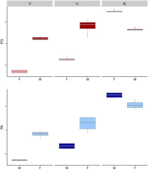
independ-ent molecular datasets on multiple populations of five sparid species: higher Nˆe estimates were obtained for the protandrous species (with the exception of one population of D. sargus), but not all the estimates from the two protogynous species available (which do not fully correspond to the species used for the life-history modelling) conformed to the expectation of low Nˆe values: indeed, while C. puniceus (with a lek-like system where males defend territories) presented low Nˆe for the majority of the populations, both populations of P. erythrinus pre-sented high value of Nˆe, comparable with the ones obtained in protandrous species (Fig. 4; Table 3). Even with estimates obtained from life history tables, the Ne estimate for this species was higher than the other species under
consideration (Fig. 2; Table 2). Pagellus erythrinus are group-spawners: their Vk* is not as high as haremic species,
but a protogynous sex change is still advantageous in this case: being a large male can be beneficial in the spawn-ing area31, 32, where the lack of haremic structure removes the typically reduced level of sperm-competition which
is the norm in protogynous species33. Furthermore, the pronouncedly lower-than expected V
k in P. erythrinus,
may to some extent stem from increased levels of female fecundity and/or k, or a possible unexplored greater contribution of primary males34, which the standardised approach we employed (see Methods) would not be able
to account for.
To test the possible interplay between sex-changing system and reproductive mode, we used two more data-sets available for two protogynous groupers, the group-spawner E. guttatus and the haremic C. fulva9: indeed, the
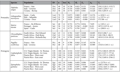
Species Population ID n loci Ho He Fis AR Nˆe
Protandry
Diplodus sargus
France – Sète Italy – Livorno Croatia – Rovinj
Ds1 Ds2 Ds3 49 49 50 10 10 10 0.738 0.754 0.776 0.822 0.826 0.831 0.121 0.089 0.061 15.094 15.222 14.428 239.5 (129.3–1155.7) 1447.1 (293.7–∞) 556.3 (205.9–∞)
Lithognathus mormyrus
Spain – Cadiz Italy – Sabaudia Croatia – Duce
Lm1 Lm2 Lm3 70 22 26 9 9 9 0.873 0.838 0.821 0.869 0.828 0.812 −0.007 −0.016 −0.008 14.576 12.333 10.455
∞ (636.5–∞)
∞ (237.6–∞) 372 (88–∞)
Sparus aurata
France – Ile d’Oleron Portugal – Aveiro Spain – Cadiz
Sa1 Sa2 Sa3 40 50 34 12 12 12 0.755 0.778 0.772 0.774 0.768 0.785 0.016 −0.002 0.017 7.829 8.421 7.911
∞ (183.2–∞) 1875.5 (237.8–∞)
∞ (200.8–∞)
Protogyny
Chrysoblephus puniceus
South Africa - Port Edward South Africa - Park Rynie South Africa - Richards Bay
Cp1 Cp2 Cp3 43 43 39 11 11 11 0.782 0.810 0.790 0.827 0.831 0.830 0.048 0.025 0.040 18.005 18.161 18.00
834.9 (286.7–∞) 128.2 (96.3–186.5) 165.8 (113.8–291.6)
Pagellus
erythrinus France – Sète Italy - Livorno Pe1 Pe2 48 48 9 9 0.700 0.701 0.843 0.877 0.145 0.188 10.556 10.989 ∞15325.4 (183.1– ∞)
Cephalopholis fulva
U.S. Virgin Islands - St. Thomas U.S. Virgin Islands - St. Croix Puerto Rico - West coast Puerto Rico - East coast
Cf1 Cf2 Cf3 Cf4 106 110 100 100 24 24 24 24 0.516 0.538 0.546 0.526 0.523 0.537 0.550 0.527 0.022 0.003 0.014 0.000 9.194 9.660 9.552 9.547 673.2 (402.9–1855.9) 465.3 (327.7–777.6) 574.1 (371.3–1199.5) 776.2 (449.4–2546.1) Epinephelus guttatus
U.S. Virgin Islands - St. Thomas U.S. Virgin Islands - St. Croix Puerto Rico - West coast Puerto Rico - East coast
Eg1 Eg2 Eg3 Eg4 101 101 95 100 19 19 19 19 0.684 0.682 0.701 0.691 0.693 0.692 0.697 0.694 0.006 0.010 −0.009 0.006 14.697 15.093 14.526 14.983
∞ (2179.4–∞) 1083.5 (594.3–5209) 1254.1 (647.3–13093.9) 2944.2 (979.7–∞)
Table 3. Genetic diversity parameters (n = sample size; loci = number of microsatellite loci) for multiple populations (with relative ID) of each species. Ho= observed heterozygosity; He= expected heterozygosity;
[image:8.595.133.554.44.297.2]www.nature.com/scientificreports/
former exhibited values similar to P. erythrinus, while the latter showed estimates comparable to C. puniceus, thereby revealing an additional layer of complexity to the scenario: we detected a decrease of Nˆe along a gradient of reproductive modes (Fig. 4) and found that harem-spawners protogynous species have lower Nˆe than group-spawning ones. Thus, behavioural traits contribute to a fuller understanding of the patterns of Ne and Vk*
in sequential hermaphrodites.
Overall, the estimates from life history tables confirmed the theoretical expectation that, in general, regardless of the direction of sex change, individuals use the same overall strategy, producing less offspring ( ) with less k¯
variance in reproductive success (Vk) as the first sex and more offspring with higher Vk as the second sex, later in
life. Concurrently, at the population level, the majority of breeders (Nb) reproduce as the first sex. Although this
trend is consistent in the two mating strategies (protandry and protogyny), its magnitude is much higher in pro-togynous species, resulting in a stronger reduction of Ne at the population level. Thus, the direction of sex change
has an influence on the overall Ne of the populations and combining all sex-changing fish species in one category
is ultimately incorrect and can be misleading for conservation and management practices.
A second independent analysis, based on molecular data also indicated that a protogynous mating system is prone to more significant reductions of Nˆe than a protandrous system. Moreover, this second analysis uncovered the fact that, in protogynous populations, Vk* may also be dependent on reproductive modes (from aggregate- to
harem-spawning) and Nˆe can change accordingly. The comparison, within protogynous sex-changing modes, between group-spawners and haremic species confirms the importance of considering and assessing the influence of mating systems and reproductive modes, in order to understand the demography of populations35. The
possi-bility that several natural stocks of haremic protogynous species may owe their persistence to a disproportionately small number of extremely successful old males fits with recent concerns regarding many valuable warm-water Figure 5. Effective population size (Nˆe) estimates, obtained with LDNe for multiple populations of the seven species under study. Bars in the tones of blue: protandrous species; bars in the tones of orange: protogynous species. (A) ˆ Nˆe values (up to infinite); (B) 1/Nˆe (note the reverse y axis as an aid to visualize Nˆe values - higher
N
[image:9.595.158.551.45.445.2]fisheries worldwide36, and calls for the practical consideration, not only of sex change, but also of its direction and
the behavioural structure underpinning it, in the management arena. Future analyses should focus on the evalu-ation of the consequences of increased mortality by fishing pressure and the populevalu-ations’ compensatory capaci-ties37. Following this path can significantly expand our ability to predict the viability of many commercially
exploited reef-associated species in tropical and warm-temperate areas, and enable us to do something useful for their preservation.
Materials and Methods
Choice of species.
Four protandrous and four protogynous species were selected (Table 1), based on existing knowledge of their biology, to produce realistic life history tables. Six of them belong to the Sparidae, a very heter-ogeneous family in terms of reproductive styles38, which includes both protandrous and protogynous species. Wepreviously generated genetic data for five out of these six sparid species, which we used in our molecular analysis (Table 3), in the attempt to minimize the biases that may arise comparing phylogenetically distant taxa. Two more protogynous species9, characterized by different social structures (aggregate- and harem-spawners) were also
included in the analysis.
Theoretical modelling.
Key life history parameters (Table 1) were retrieved from the literature and fed into a demographic model21, implemented in the freely available software AgeNe, version 2.0 (http://conserver. iugo-cafe.org/node/2876). For each species, Leslie matrices were built and age-specific survival (sx), fecundity andsex ratios were calculated.
Age-specific survival rates. Natural mortalities (m) were calculated for length classes following Charnov and colleagues39
=
− .
·
(
)
m L L/ inf 1 5 K (1)
where Linf is the asymptotic length (in cm), L is the fish standard length (in cm) and K is the growth coefficient of
the von Bertalanffy equation:
= − − −
Lx Linf(1 e( K x x( 0))) (2)
where Lx is the fish total length (in cm) at age x, and x0 is the theoretical age at length = 0. Length classes were
assigned to age classes (eq. 2) and length values for each class were compared with known data from the literature, to ensure realistic estimates. Natural instantaneous mortalities were then transformed in annual mortality rates per year (d40) using the formula:
= − −
d 1 e m (3)
To prevent survivorship in the oldest age class, age-specific survival rates were calculated as:
= − . − − ⋅ − .
sx sA (0 5/ )x {[e(x sA)] sA (0 5/ )}x (4)
which is based on a generally accepted type III survivorship curve, where sA is the asymptotic maximum survival
(s= 1 −d= e−m, from eq. 3) and x is the age. This introduced senescence reduces the adult population to zero at
the maximum age (as reported in the literature). Equation 4 adjusts survival for age, following the rationale that natural mortality increases exponentially with age24, 41. Thus, survival increases with size until at a certain age and
then decreases in older fish till all fish are dead in the oldest age class. Based on greater availability of bibliographic information, combined data for the two sexes were used. Even though this is a simplification42, the assumption
of size-dependent (and not sex-dependent) survival rates should not significantly alter the results. Indeed, for the majority of individuals (excluding the ones which do not change sex, i.e., primary males in protogyny and primary females in protandry) sex is correlated with size. This means that male survival can be assumed to be the same as female survival, but this value changes with the size of the fish39, 43. Average mortality data (across all size
classes) were compared to known mortality rates from literature, to ensure realistic estimates (Table S3).
Age-specific fecundity. Female fecundity can be calculated with an allometric (power function) relationship44–46
α
= β
( )
N LFemale fecundity eggs (5)
where α and β are constant. Surprisingly, not many data on fecundity are available from the literature. We used the data available and extrapolated the missing data, comparing calculated ranges of fertility with known ranges from literature (when available), to ensure realistic estimates (Table S3). From a practical standpoint (count of gametes), it is more difficult to calculate male fecundity. Following Alonzo and Mangel45, 46 we considered male
fecundity as 1000 times female fecundity.
Age-specific sex ratio in the population. The sex ratio in the population changes with the size of the individuals46
and thus it is different among age-classes. Individuals change sex at a specific age (tc). The proportion of the
ter-minal sex (S; males in protogynous species and females in protandrous species) was calculated with the formula:
= +
(
−)
{
+ − −}
www.nature.com/scientificreports/
where Si is the proportion of non sex-changing individuals (primary males in protogynous species and primary
females in protandrous species) and Sf is the final proportion of the terminal sex (overall sex ratios for each
spe-cies are reported in Table S3).
Given these age-specific parameters (age-specific survival rate sx; birth rate bx and sex ratio), AgeNe can
pro-duce complete life history tables for each sex, with estimates of total number of individuals in the population (total N) and estimated number of adults (adult census size N), generation length (GL i.e., the average age of parents of a newborn cohort, in years), lifetime Vk*, Ne, and annual number of breeders (Nb). Moreover, the
soft-ware estimates annual Vk, annual mean number of offspring (k¯) and annual Nb for each sex. We searched
pub-lished literature to obtain realistic parameters for our models. We are aware that a great deal of local variation exists in these parameters47, 48 and we acknowledge that geographically targeted predictions should be made for
individual populations. Here, we used data from FishBase49 to insure general (and not locality-specific) estimates
(Table 1). We checked that our life tables reproduced realistic scenarios and we made changes only when recent articles reported higher maximum length than originally reported in FishBase; Table S3). Our goal was to obtain a general (and not local) estimate of Ne, for comparative purposes among species characterized by different
mat-ing systems.
Molecular analysis.
Samples were genotyped using microsatellite loci (Table S4) run on ABI 3130xl Genetic Analyzer capillary sequencers (Applied Biosystems©). Markers were amplified using fluorescent primers labelled with 6-FAM, NED, PET and VIC dyes (Applied Biosystems©). For S. aurata, we used 12 of the 15 loci used in the original study23, since we removed three possible candidates for directional or balancing selection. Data wereanalysed with MICRO-CHECKER50 to check for large allele drop out and scoring errors; frequencies of null
alleles were estimated using the software FreeNA51. We retained loci with moderate frequency (0.05 < r < 0.20)
of null alleles51. Estimates of genetic diversity, including expected (H
e) and observed (Ho) heterozygosities, allelic
richness (AR) and coefficient of inbreeding (Fis), to test for departure from Hardy-Weinberg equilibrium, were
calculated using the package hierfstat52 while pairwise F
st values and relative 99% confidence intervals were
calculated using the package DiveRsity53 both developed in R54. We also checked for the presence of
popula-tion sub-structuring using two different approaches: STRUCTURE 2.3.455, 56 and the Discriminant Analysis of
Principal Component (DAPC) as performed in the R54 package ADEGENET v 2.0.257, 58. Only adult animals
were used in the analyses. When data from more than three populations of sparids from our lab were available, we chose truly protandrous and protogynous populations (based on logistic models for size at sex change), i.e., populations with reduced frequencies of non sex-changing individuals (primary males and primary females). Molecular markers were used to calculate Ne estimates using the software LDNe59, as implemented in NeEstimator
V260 following Gilbert and Whitlock61. Rare alleles with frequencies lower than 0.02 were excluded from our
cal-culations, as suggested by Waples and Do62.
Statistical analyses.
Comparisons between protandrous and protogynous species were performed with Student’s t-test, Welch t-test, Wilcoxon and Kruskall-Wallis tests depending on the normality and equality of variance of the data. We assessed the effect of mating system (PA and PG) on the effective size ratio Ne/N andNb/N (to control for abundance), using a series of covariates (after checking for multicollinearity; Fig. S5). For
Ne/N the best linear model (Multiple R2= 0.9396, F2,5= 38.92; p = 0.0009; AIC =−18.84) included generation
length as a covariate; for Nb/N (Multiple R2= 0.9446, F3,4= 22.73, p = 0.006), the significant covariate was
maxi-mum length. A linear model was also run for the ratio Nb/Ne (R2= 0.8929, F2,5= 0.85, p = 0.004). Linear models
were fitted to annual Vk, k¯ and Nb data considering mating system and sequential sex (first vs second, regardless if
male or female) as interaction terms. All analyses and graphical output were performed using the freely available scripts within the R environment54.
Ethical statement.
Fish samples were purchased from local fishermen. All methods and protocols were carried out in accordance with relevant guidelines and regulations. Ethical approval AREC-P-10–23 was obtained from UCD, University College Dublin.Data and materials availability.
Microsatellite genotypes can be found on Dryad Digital Repository - doi:10.5061/dryad.n722g4d3 for S. aurata23; doi:10.5061/dryad.g36ch for C. puniceus12; doi:10.5061/dryad.sj894for E. guttatus and C. fulva9; genotypes for D. sargus, P. erythrinus and L. mormyrus for will be made available
upon acceptance.
References
1. Policansky, D. Sex change in plants and animals. Annu. Rev. Ecol. Evol. Syst. 13, 471–495 (1982). 2. Shapiro, D. Y. Differentiation and evolution of sex change in fishes. Bioscience 37, 490–497 (1987).
3. Warner, R. R. Sex change in fishes: hypotheses, evidence, and objections. Environ. Biol. Fishes 22, 81–90 (1988). 4. Ross, R. M. The evolution of sex-change mechanisms in fishes. Environ. Biol. Fishes 29, 81–93 (1990). 5. Avise, J. C. & Mank, J. E. Evolutionary perspectives on hermaphroditism in fishes. Sex. Dev. 3, 152–163 (2009). 6. Warner, R. R. The adaptive significance of sequential hermaphroditism in animals. Am. Nat. 109, 61–82 (1975). 7. Warner, R. R. Sex change and the size-advantage model. Trends in Ecol. Evol. 3, 133–136 (1988).
8. Ghiselin, M. T. The evolution of hermaphroditism among animals. Q. Rev. Biol. 44, 189–208 (1969).
9. Portnoy, D. S., Hollenbeck, C. M., Renshaw, M. A., Cummings, N. J. & Gold, J. R. Does mating behaviour affect connectivity in marine fishes? Comparative population genetics of two protogynous groupers (Family Serranidae). Mol. Ecol. 22, 301–313 (2013). 10. Buchholz-Sørensen, M. &Vella, A. Population structure, genetic diversity, effective population size, demographic history and
regional connectivity patterns of the endangered dusky grouper, Epinephelus marginatus (Teleostei: Serranidae), within Malta’s Fisheries Management Zone. PloS one 11, e0159864. doi:0159810.0151371/ journal.pone.0159864 (2016).
12. Coscia, I., Chopelet, J., Waples, R. S., Mann, B. Q. & Mariani, S. Sex change and effective population size: implications for population genetic studies in marine fish. Heredity 117, 251–258 (2016).
13. Warner, R. R. Mating behavior and hermaphroditism in coral reef fishes. Amer. Sci. 72, 128–136 (1984). 14. Shuster, S. M. & Wade, M. J. Mating systems and strategies. Princeton University Press (2003). 15. Allsop, D. J. & West, S. A. Sex-ratio evolution in sex changing animals. Evolution 58, 1019–1027 (2004).
16. Charlesworth, B. Effective population size and patterns of molecular evolution and variation. Nature Rev. Gen. 10, 195–205 (2009). 17. Hare, M. P. et al. Understanding and estimating effective population size for practical application in marine species management.
Conserv. Biol. 25, 438–449 (2011).
18. Wright, S. Evolution in Mendelian populations. Genetics 16, 97–159 (1931).
19. Araki, H., Waples, R. S., Ardren, W. R., Cooper, B. & Blouin, M. S. Effective population size of steelhead trout: influence of variance in reproductive success, hatchery programs, and genetic compensation between life-history forms. Mol. Ecol. 16, 953–966 (2007). 20. Nunney, L. Measuring the ratio of effective population size to adult numbers using genetic and ecological data. Evolution 49,
389–392 (1995).
21. Waples, R. S., Do, C. & Chopelet, J. Calculating Ne and Ne/N in age-structured populations: a hybrid Felsenstein-Hill approach.
Ecology 92, 1513–1522 (2011).
22. Sala-Bozano, M., Ketmaier, V. & Mariani, S. Contrasting signals from multiple markers illuminate population connectivity in a marine fish. Mol. Ecol. 18, 4811–4826 (2009).
23. Coscia, I., Vogiatzi, E., Kotoulas, G., Tsigenopoulos, C. S. & Mariani, S. Exploring neutral and adaptive processes in expanding populations of gilthead sea bream, Sparus aurata L., in the North-East Atlantic. Heredity 108, 537–546 (2011).
24. Chopelet, J. Population Genetic Consequences of Sex Change in Marine Fish. PhD Thesis, University College Dublin (2010). 25. Munday, P. L., Kuwamura, T. & Kroon, F. J. Bidirectional sex change in marine fishes. In: Reproduction and Sexuality in Marine
Fishes: Patterns and Processes (ed K.S. Cole) University of California Press, pp. 241–271 (2010).
26. Vindenes, Y. & Langangen, Ø. Individual heterogeneity in life histories and eco-evolutionary dynamics. Ecol. Lett. 18, 417–432 (2015).
27. Lowerre-Barbieri, S. et al. Reproductive resilience: a paradigm shift in understanding spawner-recruit systems in exploited marine fish. Fish Fish. doi:10.1111/faf.12180 (2016).
28. Waples, R. S., Luikart, G., Faulkner, J. R. & Tallmon, D. A. Simple life-history traits explain key effective population size ratios across diverse taxa. Proc. R. Soc. Lond. B 280, 20131339 (2013).
29. Waples, R. S. & Antao, T. Intermittent breeding and constraints on litter size: consequences for effective population size per generation (Ne) and per reproductive cycle (Nb). Evolution 68, 1722–1734 (2014).
30. Hedrick, P. Large variance in reproductive success and the Ne/N ratio. Evolution 59, 1596–1599 (2005).
31. Coelho, R. et al. Life history of the common pandora, Pagellus erythrinus (Linnaeus, 1758)(Actinopterygii: Sparidae) from southern Portugal. Braz. J. Oceanogr. 58, 233–345 (2010).
32. Stockley, P., Gage, M. J., Parker, G. & Møller, A. Sperm competition in fishes: the evolution of testis size and ejaculate characteristics. Am. Nat. 149, 933–954 (1997).
33. Molloy, P. P., Goodwin, N. B., Côté, I. M., Reynolds, J. D. & Gage, M. J. Sperm competition and sex change: a comparative analysis across fishes. Evolution 61, 640–652 (2007).
34. Busalacchi, B., Bottari, T., Giordano, D., Profeta, A. & Rinelli, P. Distribution and biological features of the common pandora, Pagellus erythrinus (Linnaeus, 1758), in the southern Tyrrhenian Sea (Central Mediterranean). Helgoland Mar. Res. 68(4), 491–501 (2014).
35. Kazancıoğlu, E. & Alonzo, S. H. Classic predictions about sex change do not hold under all types of size advantage. J. Evolution. Biol.
23, 2432–2441 (2010).
36. Sadovy de Mitcheson, Y. et al. Fishing groupers towards extinction: a global assessment of threats and extinction risks in a billion dollar fishery. Fish Fish. 14, 119–136 (2013).
37. Kindsvater, H. K., Mangel, M., Reynolds, J. D. & Dulvy, N. K. Ten principles from evolutionary ecology essential for effective marine conservation. Ecol. Evol. 6, 2125–2138 (2016).
38. Buxton, C. D. & Garratt, P. A. Alternative reproductive styles in seabreams (Pisces: Sparidae). Environ. Biol. Fishes 28, 113–124 (1990).
39. Charnov, E. L., Gislason, H. & Pope, J. G. Evolutionary assembly rules for fish life histories. Fish Fish. 14, 213–224 (2013). 40. Kuparinen, A., Hutchings, J. A. & Waples, R. S. Harvest-induced evolution and effective population size. Evol. Appl. 9, 658–672
(2016).
41. Tanasichuk, R. W. Natural mortality rates of adult Pacific herring (Clupea pallasi) from Southern British Columbia. Canadian Stock Assessment Secretariat Research Document 99/168, Nanaimo, B.C., Canada, 34 pp (1999).
42. Garratt, P. A., Govender, A. & Punt, A. E. Growth acceleration at sex change in the protogynous hermaphrodite Chrysoblephus puniceus (Pisces: Sparidae). S. Afr. J. Mar. Sci. 13, 187–193 (1993).
43. Gislason, H., Daan, N., Rice, J. C. & Pope, J. G. Size, growth, temperature and the natural mortality of marine fish. Fish Fish. 11, 149–158 (2010).
44. Warner, R. R. The reproductive biology of the protogynous hermaphrodite Pimelometopon pulchrum (Pisces: Labridae). Fish. Bull.
73, 262–283 (1975).
45. Alonzo, S. H. & Mangel, M. The effects of size-selective fisheries on the stock dynamics of and sperm limitation in sex-changing fish. Fish. Bull. 102, 1–13 (2004).
46. Alonzo, S. H. & Mangel, M. Sex-change rules, stock dynamics, and the performance of spawning-per-recruit measures in protogynous stocks. Fish. Bull. 103, 229–245 (2005).
47. Hamilton, S. L., Wilson, J. R., Ben-Horin, T. & Caselle, J. E. Utilizing spatial demographic and life history variation to optimize sustainable yield of a temperate sex-changing fish. PloS one 6, e24580 (2011).
48. Mouine, N., Ktari, M. H. & Chakroun-Marzouk, N. Reproductive characteristics of Spondyliosoma cantharus (Linnaeus, 1758) in the Gulf of Tunis. J. Appl. Ichthyol. 27, 827–831 (2011).
49. Froese, R. & Pauly, D. FishBase. World Wide Web electronic publicationwww.fishbase.org ver. 08/2012 (2011).
50. Van Oosterhout, C., Hutchinson, W. F., Wills, D. P. M. & Shipley, P. Micro-checker: software for identifying and correcting genotyping errors in microsatellite data. Mol. Ecol. Notes 4, 535–538 (2004).
51. Chapuis, M. P. & Estoup, A. Microsatellite null alleles and estimation of population differentiation. Mol. Biol. Evol. 24, 621–631 (2007).
52. Goudet, J. HIERFSTAT, a package for R to compute and test hierarchical F-statistics. Mol Ecol. Notes 5, 184–186 (2005).
53. Keenan, K., McGinnity, P., Cross, T. F., Crozier, W. W. & Prodӧhl, P. A. DiveRsity: an R package for the estimation and exploration of population genetics parameters and their associated errors. Methods Ecol. Evol. 4, 782–788 (2013).
54. R Core Team R: A language and environment for statistical computing. R Foundation for Statistical Computing, Vienna, Austria.
https://www.R-project.org/ (2016).
55. Pritchard, J. K., Stephens, M. & Donnelly, P. Inference of population structure using multilocus genotype data. Genetics 155, 945–959 (2000).
www.nature.com/scientificreports/
57. Jombart, T. Adegenet: a R package for the multivariate analysis of genetic markers. Bioinformatics 24, 1403–1405 (2008). 58. Jombart, T. & Amhed, I. Adegenet 1.3-1: new tools for the analysis of genome-wide SNP data. Bioinformatics 27, 3070–3071 (2011). 59. Waples, R. S. & Do, C. LDNE: a program for estimating effective population size from data on linkage disequilibrium. Mol. Ecol.
Resour. 8, 753–756 (2008).
60. Do, C., Waples, R. S., Peel, D., Macbeth, G. M., Tillett, B. J. & Ovenden, J. R. NeEstimator V2: re-implementation of software for the estimation of contemporary effective population size (Ne) from genetic data. Mol. Ecol. Resour. 14, 209–214 (2014).
61. Gilbert, K. J. & Whitlock, M. C. Evaluating methods for estimating local effective population size with and without migration. Evolution 69, 2154–2166 (2015).
62. Waples, R. S. & Do, C. Linkage disequilibrium estimates of contemporary Ne using highly variable genetic markers: a largely untapped resource for applied conservation and evolution. Evol. Appl. 3, 244–262 (2010).
63. González-Wangüemert, M., Pérez-Ruzafa, A., Cánovas, F., García-Charton, J. A. & Marcos, C. Temporal genetic variation in populations of Diplodus sargus from the SW Mediterranean Sea. Mar. Ecol. Prog. Ser. 334, 237–244 (2007).
64. Molloy, P. P., Goodwin, N. B., Côté, I. M., Gage, M. J. G. & Reynolds, J. D. Predicting the effects of exploitation on male-first sex-changing fish. Anim. Conserv. 10, 30–38 (2007).
65. Kallianiotis, A., Torre, M. & Argyri, A. Age, growth, mortality, reproduction and feeding habits of the striped seabream, Lithognathus mormyrus (Pisces: Sparidae) in the coastal waters of the Thracian Sea, Greece. Sci. Mar. 69, 391–404 (2005).
66. Vitale, S., Arkhipkin, A., Cannizzaro, L. & Scalisi, M. Life history traits of the striped seabream Lithognathus mormyrus (Pisces, Sparidae) from two coastal fishing grounds in the Strait of Sicily. J. Appl. Ichthyol. 27, 1086–1094 (2011).
67. Kraljević, M. & Dulčić, J. Age and growth of gilt-head sea bream (Sparus aurata L.) in the Mirna Estuary, Northern Adriatic. Fish. Res. 31, 249–255 (1997).
68. Staunton-Smith, J., Robins, J. B., Mayer, D. G., Sellin, M. J. & Halliday, I. A. Does the quantity and timing of freshwater flowing into a dry tropical estuary affect year-class strength of barramundi (Lates calcarifer). Mar. Freshwater Res. 55, 787–797 (2004). 69. Kumarlal, K. & James, P. S. B. R. Egg production in the threatened seabass, Lates calcarifer (Bloch) along Tuticorin coast, Gulf of
Mannar. Indian J. Fish. 45, 451–455 (1998).
70. Garratt, P. A., Govender, A. & Punt, A. E. Growth acceleration at sex change in the protogynous hermaphrodite Chrysoblephus puniceus (Pisces: Sparidae). S. Afr. J. Mar. Sci. 13, 187–193 (1993).
71. Garratt, P. A. The offshore line fishery of Natal: II: Reproductive biology of the sparids Chrysoblephus puniceus and Cheimerius nufar. Investigational Report Oceanographic Research Institute 62, 1–21 (1985).
72. Pajuelo, J. G. & Lorenzo, J. M. Population biology of the common pandora Pagellus erythrinus (Pisces: Sparidae) off the Canary Islands. Fish. Res. 36, 75–86 (1998).
73. Pajuelo, J. G. & Lorenzo, J. M. Life history of black seabream, Spondyliosoma cantharus, off the Canary Islands, Central-east Atlantic. Environ. Biol. Fishes 54, 325–336 (1999).
74. Dulčić, J., Skakelja, N., Kraljević & Cetinic, M. P. On the fecundity of the Black Sea bream, Spondyliosoma cantharus (L.), from the Adriatic Sea (Croatian coast). Sci. Mar. 62, 289–294 (1998).
75. Loke-Smith, K. A. et al. Reassesment of the fecundity of California sheephead. Mar. Coast. Fish. 4, 599–604 (2012).
Acknowledgements
We would like to thank all researchers that contributed to the empirical studies that generated the genotypes used here for parameter estimation. The manuscript benefited from extensive and constructive comments by Prof Robin Waples. The study was funded by the Irish Research Council and Science Foundation Ireland.
Author Contributions
C.B. and S.M. designed the study, C.B. and J.C. set up the theoretical model, C.B. prepared the life history tables and run the theoretical analysis, C.B. and I.C. analysed the data and produced the figures, S.M. produced the fish drawings for Figure 1, C.B., M.S.-B., I.C. and J.C. collected genetic data, C.B., M.S.-B., I.C. and S.M. commented on study throughout, C.B. wrote the manuscript with the assistance of I.C. and S.M.
Additional Information
Supplementary information accompanies this paper at doi:10.1038/s41598-017-09298-8 Competing Interests: The authors declare that they have no competing interests.
Publisher's note: Springer Nature remains neutral with regard to jurisdictional claims in published maps and institutional affiliations.
Open Access This article is licensed under a Creative Commons Attribution 4.0 International License, which permits use, sharing, adaptation, distribution and reproduction in any medium or format, as long as you give appropriate credit to the original author(s) and the source, provide a link to the Cre-ative Commons license, and indicate if changes were made. The images or other third party material in this article are included in the article’s Creative Commons license, unless indicated otherwise in a credit line to the material. If material is not included in the article’s Creative Commons license and your intended use is not per-mitted by statutory regulation or exceeds the perper-mitted use, you will need to obtain permission directly from the copyright holder. To view a copy of this license, visit http://creativecommons.org/licenses/by/4.0/.