A Predictive Sliding Mode Cascade Controller for Nonholonomic Autonomous Systems

(1)

International Journal of Emerging Technology and Advanced Engineering

Website: www.ijetae.com (ISSN 2250-2459, ISO 9001:2008 Certified Journal, Volume 7, Issue 8, August 2017)

11

A Predictive Sliding Mode Cascade Controller for

Nonholonomic Autonomous Systems

Mansour Rostami

1

, Ali Reza Sedaghati

2

1_{MS student of Electrical Engineering, Shahabdanesh Institute of Higher Education, Qom, Iran} 2_{PhD in Electrical Engineering, Shahabdanesh Institute of Higher Education, Qom, Iran}

Abstract— This paper presents several nonlinear control

applications for nonholonomic autonomous wheeled mobile robot and unmanned surface vessel (USV) systems. First, an overview of nonlinear control and nonholonomic systems is given and sliding mode control (SMC) and model predictive control (MPC) methods are introduced. Next, a kinematic controller is applied to an experimental wheeled mobile robot for validation of rapid prototyping techniques and new trajectory planning algorithms. Then, SMCs are developed for set point and trajectory tracking of USVs. The SMC provides a robust control law with modest computational requirements that can be implemented on small-scale model USV systems. However, tuning the control parameters can be very non-intuitive and one set of parameters is rarely suitable for different initial conditions. Finally, a predictive sliding mode cascade controller is developed combining the strengths of the sliding mode and MPC methods. Simulation and/or experimental results are presented for each application.

Keywords— Nonholonomic Systems, Model Predictive Control, Sliding Mode Control, Cascade Control.

I. INTRODUCTION

Autonomous systems have received increased attention in the last decades as the need arises for mechanical systems to perform tasks in situations where it may be too difficult or dangerous for a human. The term autonomous systems in this context refers to mobile systems that carry out predefined tasks without human input or control, i.e., mobile robots, unmanned surface or underwater vessels, unmanned air vehicles, etc. These systems are becoming more widely desired for military and industrial applications and as a result, there is a great deal of current research focused on control methodologies that allow these systems to carry out their tasks in the often unstructured and unpredictable environments in which they are used [1].

Many autonomous systems can be considered as underactuated mechanical systems [2]. Underactuated systems are defined as systems containing fewer inputs than degrees of freedom. Most of these underactuated systems are subject to first- or second-order nonholonomic constraints defined in terms of system velocities or accelerations respectively [3].

Nonholonomic systems present interesting control problems that require a variety of solutions ranging from

relatively simple kinematic controllers to more

sophisticated nonlinear controllers depending on the type of system, the application and the environment [4]. This paper focuses on the control of two types of nonholonomic autonomous systems: the differential drive wheeled mobile robot and the autonomous unmanned surface vessel (USV). Wheeled mobile robot systems have many real-world applications because they are a very useful and practical platform for both military and industrial purposes. Also, because of its simplicity, this type of system is an excellent platform for educational and research applications. The system presented in this thesis employs a simple kinematic control law is used for experimental validation of new rapid-prototyping techniques and trajectory planning algorithms.

Position control of wheeled mobile robots is a fairly well established area of research with much of the literature focused on kinematic control techniques. In general, position control of mobile robots can be divided into setpoint [5, 6] and trajectory tracking [7,31] control where the formulation of the corresponding control law can be very different depending on the intended application. In [11], implementation of the factitious force concept for a controlling complex mobile manipulator has been presented. The method of factitious force assumes extension on the dynamics level, in the form of an additional control inputs uv, which values are equal to zero equivalently. For a mobile manipulator, consisting of platform REX and 5R robotic onboard arm, a cascaded

control law has been proposed. A combined

kinematic/torque control law developed using backstepping and applied to both trajectory tracking and setpoint stabilization is presented in [12].

Position control of autonomous USV systems is also a very active area of research which has received increased attention in the last decade with most of the research

focusing on feedback linearization, backstepping,

(2)

International Journal of Emerging Technology and Advanced Engineering

12 As with control of mobile robot systems, the USV control problems can be divided into setpoint position [13– 18] and trajectory tracking [19–27] control. In this paper, several examples of nonlinear control laws for the USV setpoint and trajectory tracking control problems are presented. First, SMCs are presented for tracking [27] and setpoint control [28]. The advantage of these controllers is that they require very little computation and can be implemented on the small scale model USV system. A disadvantage of these controllers, however, is that tuning the control parameters can be very non-intuitive and often the optimal parameters for one initial condition can yield poor performance given different initial conditions. Next, a new MPC method is applied to trajectory tracking and setpoint control [29, 30]. MPC is based on solving an open-loop optimal control problem at each sampling instant. As a result, open-loop optimal performance can be achieved regardless of initial conditions, constraints or disturbances. Another advantage of this method is that the setpoint and trajectory tracking controllers use the same formulation. The disadvantage, however, is that the controller requires significant computation time making it challenging to implement on-line for small scale USV systems with relatively fast dynamics. Therefore, a cascade MPC and SMC is presented which effectively combines the fast computation of the sliding mode tracking controller with the optimal performance of the MPC.

II. NONLINEAR AND NONHOLONOMIC SYSTEMS

A. Nonlinear Control

Linear control is a very well developed subject with many relevant and successful applications for systems whose behavior in the desired operating ranges can be accurately described by these linear approximations. However, if the required operating range is large or the system is too nonlinear, linear control techniques are likely to break down as they fail to compensate for the nonlinearities of the true system. For these systems, nonlinear control techniques may provide greatly increased performance and stability. In the case of underactuated nonholonomic systems, nonlinear control methods are more appropriate because the nonholonomic constraints are inherently nonlinear.

Many techniques have been developed for solving both nonlinear setpoint and nonlinear tracking control problems. These techniques include feedback linearization, adaptive control, gain scheduling, SMC, MPC and robust control. The equation of motion for control-affine time-varying nonlinear dynamic systems is given by

( , ) ( ) , ( )

x f x t g x u

y h x

 

 (1)

The purpose of control system design is to define a control law u(x, t) such that x → 0 in the case of set point control, or y→yd(t) in the case of tracking control, where yd(t) is the desired output trajectory. Many simple, time-invariant and fully actuated problems may be solved by designing the control law in such a way as to cancel the nonlinear dynamics of the plant, f(x), leaving the closed-loop system in a linear form resembling that shown in Eq. (2) such that linear control techniques can be applied.

,

x Ax Bu

y Cx

 

 (2)

This type of control system design is known as feedback linearization and should not be confused with conventional linearization. In the case of feedback linearization, the complete nonlinear model in conjunction with state feedback is used to transform the system into a linear form, whereas the latter technique makes a linear approximation of the system about a given equilibrium point. Feedback linearization can be used to derive linear control systems for many nonlinear dynamic systems but cannot be applied universally. Some disadvantages of feedback linearization are that it requires full state feedback and it is not robust to modeling uncertainty or unmodeled dynamics. In this paper, nonlinear sliding mode and MPCs are introduced and several applications are presented.

B. Nonholonomic Systems

Underactuated mechanical systems, i.e., systems containing fewer inputs than degrees of freedom (DOF), are also examples of nonholonomic systems. Consider an n-DOF mechanical system under the action of m < n, m ≥1 control inputs, u ϵ Rm, where the set of generalized coordinates of the system is denoted by q = (q1, …, qn). The set of generalized coordinates is partitioned as q = (qa, qu)

where the vector qa ϵ Rm represents the actuated

coordinates and the vector qu ϵ Rn-m represents the unactuated coordinates. The equations of motion of the underactuated system can thus be expressed as

( ) ( ) ( , ) ( )

11 12 1

M q q_aM q q_uF q q B q u (3)

( ) ( ) ( , ) 0

21 22 2

M q q_aM q q_uF q q  (4)

(3)

International Journal of Emerging Technology and Advanced Engineering

13 Assuming they are nonintegrable, Eq. (4) define n-m second order nonholonomic constraints.

C. Kinematic Control for Mobile Robots

A typical example of an underactuated system with a first-order nonholonomic constraint is the differential-drive wheeled mobile robot. Mobile robot technology is widely used in military and industrial environments and the differential drive configuration is one of the most simple and widely used mobile robot platforms. Also, because this configuration is relatively simple both to manufacture, and model mathematically, it is used quite often in education and research environments to develop or demonstrate mobile robot technology.

D. Kinematic Model

The differential-drive wheeled mobile robot consists of two independently actuated front drive wheels of radius r mounted on a common axis as shown in Fig. 1. The track width l represents the length of the segment connecting the wheel centers. A passive caster supports the rear of the mobile robot. The 3-DOF planar posture of the robot is described in the inertial reference frame by the vector p= [x, y, θ] T and the motion of the mobile robot is subject to the first-order nonholonomic constraint

cos sin 0

y x  (5)

Assuming that the wheels do not slip. The planar motion is described by the velocity vector q = [v ω] T where v is the forward velocity of the robot in the direction orthogonal to the drive wheel axis and ω is the angular velocity of the robot about the center of the drive wheel axis. The kinematic equations relating the body fixed velocities q to the inertial

cos 0

sin 0

0 1

x

v y

 

 



  

_{  }

  

_{  }

 

  



  



(6)

The body fixed velocities are related to the angular velocities of the drive wheels by

2 2

r r

v _R

r r _L

l l



  







  

 



  

 

 

_

_

 





(7)

[image:3.612.348.548.169.349.2]

where ωL and ωR are the angular velocities of the left and right wheels respectively.

Fig. 1. Differential drive mobile robot schematic

E. USV System Model

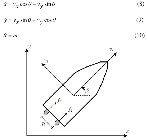
[image:3.612.320.558.454.681.2]

The 3-DOF planar model of a surface vessel shown in Fig. 2 is considered. This model includes surge, sway, and yaw motion with two propeller force inputs f1 and f2. The geometrical relationship between the inertial reference frame and the vessel-based body fixed frame is defined in terms of velocities as

cos sin

xv_x v_y  (8)

sin cos

yv_x v_y  (9)

  (10)

(4)

International Journal of Emerging Technology and Advanced Engineering

14 where x and y denote the position of the center of mass, θ is the orientation angle of the vessel in the inertial reference frame, vx and vy are the surge and sway velocities, respectively, and ω is the angular velocity of the vessel.

In the body-fixed frame, the nonlinear equations of motion for a simplified model of the dynamics of a surface vessel, where motion in heave, roll, and pitch are neglected, are given by

( )

11 22

m v_xm v_yg_x v_x  f (11)

( ) 0

22 11

m v_y m v_xg_y v_y  (12)

( ) 33

m m v v_d _{x y}g_z  T (13)

where mii are the mass and inertial parameters, md = m22-m11>0 andg x y z{ , , }are the hydrodynamic drag forces on the vessel in each axis of motion. The mii parameters include added mass contributions that represent hydraulic pressure forces and torque due to forced harmonic motion of the vessel which are proportional to acceleration. In this paper, only forward vessel motion, vx > 0, is considered because the forward and reverse motion dynamics are quite different. The surge control force f and the yaw control moment T are given in terms of the two propeller forces as

1 2

( ₂ ₁) / 2

f f f

T B f f

 

  (14)

where B is the lateral distance between the propellers. The unactuated equation of motion (12) is interpreted as a second-order nonholonomic constraint.

III. NONLINEAR CONTROL AND NONHOLONOMIC SYSTEMS

The unmanned surface vessel system is a nonholonomic system. The control problems considered using these methods can generally be divided into setpoint position [1,2] and trajectory tracking [3,4] control.

A. Partial Feedback Linearization

The two inputs of the system are redefined to be the

angular and surge accelerations,   and _vx ,

respectively

( ( ) ) /

1 22 11 33 33

u  T m m v v_{x y}d  m (15)

( ) /

2 22 11 11

u  f m v_yd v_x m (16)

where u1 is the angular acceleration and u2 is surge acceleration. The first three states of the model are defined as the vessel orientation angle and the body-fixed coordinates of the vessel center of mass

1

s

x    (17)

( ) cos ( ) sin

2

s s

x  xx  yy  (18)

( ) sin ( ) cos

3

s s

x   x x  yy  (19)

where (xs, ys, θs) represent the desired position and orientation setpoint of the vessel. Three additional states are defined as the vessel’s sway, angular, and surge velocities.

4

x _{v y} (20)

5

x    (21)

6 x

x



v

(22)

B. SMC for Unmanned Surface Vessels

A setpoint SMC law is developed using four sliding surfaces for calculation of the two propeller forces. The yaw moment control is developed by defining a sliding surface for orientation stabilization. The surge control is derived by defining three additional surfaces. The trajectories are proved to converge to the first surface at a finite time and the remaining three surfaces simultaneously at a different finite time. Finally,the sliding phase is shown to be asymptotically stable through the introduction of a Lyapunov function.

Finite time control concepts introduced in [8, 9] are used to develop a control law that guarantees system trajectories reach all sliding surfaces in finite time. Hence, the trajectories are asymptotically stabilized due to the linear stable nature of the surfaces. The first asymptotically stable sliding surface is defined as

, 5

1 1

s x x 0 (23)

In order to stabilize the vessel orientation. The control law that pushes all trajectories to this surface can be calculated using the finite time approach

1

sgn( ) ₅,

1 1 1 1

(5)

International Journal of Emerging Technology and Advanced Engineering

15

C. SMC Law

The USV model inputs are calculated by solving for the yaw moment and surge force in Eqs. (23) and (24) respectively

( )

33 1 22 11 33

T m u  m m v v_{x y}d  (25)

11 2 22 11

f m u m v_yd v_x (26)

Finally, the individual propeller inputs are calculated by inverting Eq. (14).

1 / 2 1 / 1

1 / 2 1 / 2

f B f

f B T

 



  

  

  

_

  

_{  }

 

(27)

1) Results

The control parameters are selected as

1.1, 2, 1, 1, 1 / 2

3 2 1 1 2

         

In addition, it is assumed that the boat propellers are

only able to produce maximum surge force of fmax = 1.18 N

and yaw moment of Tmax = 0.06 Nm. These saturation limits are not accounted for in the simulations but are present in the experiments. The controller performance is evaluated in simulation and experimentally through two setpoint problems. In both cases the USV begins at rest at an initial position and orientation determined by the camera.

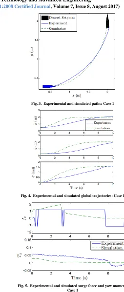
For the first example, the initial position of the boat is determined to be (0 4 m, 0 2 m, 0 ) and the desired setpoint is (2m, 2m, 0 ) Fig 3 shows that the experimental and simulated USV paths are similar though with some difference.

The difference becomes more pronounced when the x, y and θ time histories are plotted as in Fig 4 It is clear that x and θ stabilize fairly accurately but y position does not fully stabilize in the experiment due to a small forward velocity at the desired setpoint. The reason for this problem is the saturation limits which cut off the surge force significantly, as shown in Fig. 5.

[image:5.612.295.549.116.715.2]

The experimental error may also be partially due to camera calibration and model errors [4]. Fig. 6 shows the simulated time history of the four surfaces where the surface reach times are τ1 = 2 2 s and τ2 = 4 s.

[image:5.612.355.534.128.519.2]

Fig. 3. Experimental and simulated paths: Case 1

Fig. 4. Experimental and simulated global trajectories: Case 1

(6)

International Journal of Emerging Technology and Advanced Engineering

[image:6.612.67.277.119.292.2]

16

Fig. 6. Simulated time history of the four surfaces: Case 1

D. Trajectory Tracking Control

In this section, a trajectory tracking SMC law for autonomous surface vessels is developed using two sliding surfaces for calculation of the two propeller forces [4]. The first sliding surface is a first-order surface defined in terms of the surge motion tracking errors. The second sliding surface is a second-order surface defined in terms of the lateral motion tracking errors. Hence, the absolute velocities are numerically estimated, and surge and sway velocities are calculated through kinematic relations between inertial and body-fixed reference frames. The desired state trajectories in the inertial reference frame are related to the corresponding surge and lateral velocities as follows

cos sin

1 2

r

v_x x x  (28)

sin cos

1 2

r

v_y  x x  (29)

1) Results

[image:6.612.349.535.120.328.2]

In the following simulation example, a target follows a circular trajectory centered at (x = 1m, y = 2m) with a radius of 0.5 meters and constant angular velocity of 0.2 rad/sec (a period of about 30s) beginning at (x = 1.5m, y = 2m). The USV must approach and track the target from an initial position at (x = 2m, y = 2m) represented by the boat icon in Fig. 7.

Fig. 7. Simulated USV path: trajectory tracking SMC

[image:6.612.326.562.427.527.2]

The control parameters are selected as λ1 = λ2 = 1, ε1 = ε2 = 0 05 and η1 = η2 = 0.2. The target and USV paths are presented in Fig. 7 and the control action is presented in Fig. 8. As shown in these figures, the control action is feasible and the USV reaches the target in a reasonable amount of time.

Fig. 8. Control input: trajectory tracking SMC

E. MPC for Unmanned Surface Vessels

(7)

International Journal of Emerging Technology and Advanced Engineering

17

F. MPC

The MPC strategy attempts to achieve a specified performance objective in an optimal manner by solving a finite horizon, open-loop optimal control problem online at each control interval. The algorithm computes the control inputs u that minimize the objective function over the prediction horizon N. The first input u1 is implemented for one control interval and the process is repeated given the new initial conditions of the system. This technique is referred to as receding horizon control.

A finite horizon performance objective following the Lagrange cost function in optimal control [10] is used



min,...,



( ) ( , , )

1

k N t

J_k _{k t} z u t dt

u _un

 

_{ }  (30)

[image:7.612.56.284.424.507.2]

As opposed to holding the value of each future input for a single control interval in the prediction horizon, an input or move blocking strategy [5,31] is employed where each future input move is held constant over several control intervals within the prediction horizon. The advantage of this approach is a reduction in the number of future control moves (optimization decision variables) that must be determined such that n << N.

Fig. 9. Control input vector parameterization

1) Results

The trajectory and setpoint control examples are based on the problem of recovering an autonomous USV using a stern recovery ramp on a target vessel [12] whose position and orientation are denoted by xt, yt and θt. The initial recovery phase, in which the USV must converge to the target vessel trajectory or position, is considered in the examples presented in this chapter. The performance objective used in these examples is a quadratic penalty on the distance from the target trajectory and the desired orientation or heading angle

2 2

( , , )z u t _dd t( )  _a( ( )t _d( , ))t d

    (31)

2 2 2

( ) ( ( ) ( )) ( ( ) ( ))

d t x t x t_t  y ty t_t (32)

where θd is the desired USV orientation and d is the distance between the USV and the target.

The trajectories using linear drag force model are indicated by a dot-dash line in the same figures. The linear drag force is the more common form used in USV dynamic modeling [6–7] and results in stable linear trajectories, but it is only really appropriate at very low velocities.

G. Linear Target Trajectory Tracking

In this example, the recovery vessel is following a linear path with a constant velocity. The USV must first approach the recovery vessel and then track its trajectory. The following performance objective parameters are used

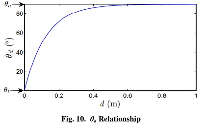
1, a d

   _d( , )t d _ted _a(1ed) (33)

where the desired USV orientation angle θd is a function of the target vessel orientation angle θt and the angle of the line between the USV and the target vessel θa In order to obtain reasonable tracking trajectories, the USV orientation angle should approach θa when it is far away from the target and approach the target orientation angle when it is close to the target. This behavior is produced by the exponential relationship in Eq. (33) as shown in Fig. 10 with θt = 0 , = and θa = 0

Fig. 10. θaRelationship

The control and prediction horizons are n = 2 and N = 10 with a control period of Δt =0.2s. The control move is parameterized within the prediction horizon as

, ( )

1 1

( )

, ( ) ( )

2 1

u k t t k j t

u t

u k j t t k N t

    



     







where j1=5. In order to improve the tracking

performance and prevent the USV from colliding with the target vessel with this short control horizon, the following state constraints

0,

y_yt_y 

  _t  0,

x x 0 t x

[image:7.612.341.547.430.556.2]

(8)

International Journal of Emerging Technology and Advanced Engineering

[image:8.612.53.539.109.635.2]

18

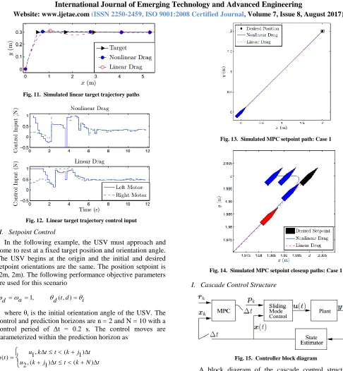
Fig. 11. Simulated linear target trajectory paths

Fig. 12. Linear target trajectory control input

H. Setpoint Control

In the following example, the USV must approach and come to rest at a fixed target position and orientation angle. The USV begins at the origin and the initial and desired setpoint orientations are the same. The position setpoint is (2m, 2m). The following performance objective parameters are used for this scenario

1, a d

  

_d( , )t d _i

where θi is the initial orientation angle of the USV. The control and prediction horizons are n = 2 and N = 10 with a control period of Δt = 0 2 s The control moves are parameterized within the prediction horizon as

, ( )

1 1

( )

, ( ) ( )

2 1

u k t t k j t

u t

u k j t t k N t

    



     







where j1=1. In order to prevent overshooting the desired position target, the following inequality constraints are also applied

0,

x_xt_x 

y_yt_y 0

Fig. 13. Simulated MPC setpoint path: Case 1

Fig. 14. Simulated MPC setpoint closeup paths: Case 1

[image:8.612.70.266.251.414.2]

I. Cascade Control Structure

Fig. 15. Controller block diagram

[image:8.612.326.553.512.612.2]

(9)

International Journal of Emerging Technology and Advanced Engineering

19 For this application, the control interval tdoes not need to be fixed. The SMC computes the control input to the USV system at a rate sufficient to stabilize the system. The MPC is based on a finite horizon performance objective following the Lagrange cost function in optimal control [10] similar to Eq. (30)

( )

minJ_k _{k t}k N t ( , , )z u t dt p

 

_{ }  (34)

where Jk is the objective function value at sample time Δt and k is the control interval, N is the prediction horizon, Φ(∙) is the performance penalty function, z is the state of the system and u is the propeller forces determined by the SMC. This objective is minimized over the surface, effort and trajectory parameters p subject to the following constraints

( , , )

z f z u t (35)

1

1 1

1

/ 2 / 2 2

f f

u

f B B T



 



  

  

  

_

  

_{  }

 

(36)

( , ) 0

g z u  (37)

( ) 0

h p  (38)

where f(x, u, t) are kinematic and dynamic equality constraints arising from the USV system model Eqs. 8-13, g(z, u) is a general inequality constraint on the states and control, and h(p) is a general inequality constraint on the controller parameters arising from the surface and trajectory derivation. Eq. (36) determines the individual propeller forces as a function of surge force f and yaw moment T.

J. Simulations Results

USV system dynamic equations is defined as follows

( ). ( , ). ( )

M q qV q q qG q   (39)

By applying the dynamic equations to the system states we have

2 ( ). ( ).[ . ] ( ).[ ] ( ) M q q B q q q C q q G q

     (40)

Three links used in this paper are defined as follows

0 5

4 6

q q q 

2 ( ). ( ).[ . ] ( ).[ ] ( ) A q q B q q q C q q G q

     (41)

matrix A is symmetric and 6 * 6

0 0 0

11 12 13

0 0 0

21 22 23

0 0

31 32 33 35

( )

0 0 0 ₄₄ 0 0

0 0 0 0 ₅₅ 0

0 0 0 0 0 ₆₆

a a a

a a a a

A q a a a                      (42)

and matrix B is

0 0 0 0 0 0 0 0 0 0 0

112 113 115 123

0 0 ₂₁₄ 0 0 ₂₂₃ 0 ₂₂₅ 0 0 ₂₃₅ 0 0 0 0

0 0 ₃₁₄ 0 0 0 0 0 0 0 0 0 0 0 0

( )

0 0 0 0 0 0 0 0 0 0 0 0

412 413 415

0 0 ₅₁₄ 0 0 0 0 0 0 0 0 0 0 0 0

0 0 0 0 0 0 0 0 0 0 0 0 0 0 0

b b b b

b B q

b b b

b                      (43)

and matrix C

0 ₁₂ ₁₃ 0 0 0

0 0 0 0

21 23

0 0 0 0

31 32

( )

0 0 0 0 0 0

0 0 0 0

51 52

0 0 0 0 0 0

c c c c c c C q c c                      (44)

and matrix G

( ) 0 ₂ ₃ 0 ₅ 0

g q 





g g g





. 2 . 23 . 2 . 23 ₅. 23

2 1 2 3 4

g g C g S g S g C g S

. 23 . 23 ₅. 23

3 2 4

g g S g C g S

,

g₅g S₅. 23 (45)

1) using three links USV

For USV kinematic finding with 3-DOF, a system with D-H coordinate is designed.

2 ( ). ( ). ( ). ( ) A q q B q qq C q q g q

     and q₄  q₅ q₆ 0 (46)

2) Angular velocity





1_{( ).} _{( ).} _{( ).} 2 _{( )} qA q  _B q qqC q q g q_

 

Now let_I_{  }



_{B q qq C q q}_{( ).} _ _{( ).} 2__{g q}_{( )}



_

 

  q A 1( ).q I



(10)

International Journal of Emerging Technology and Advanced Engineering

[image:10.612.322.562.127.725.2]

20 The SMC is designed for use in MATLAB. The following figures show the system states that follows path reference. Next the MPC is employed, which is the general structure of USV. The difference is that the controller scheme in design simulator which defines as follows is changed.

Fig. 16. SMC system states

Fig. 17. SMC system states

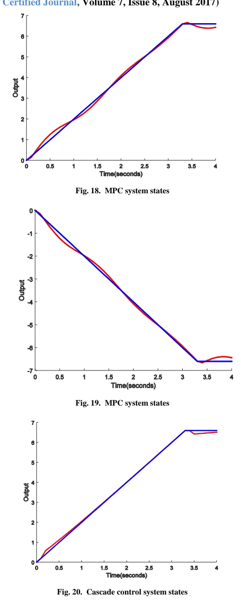
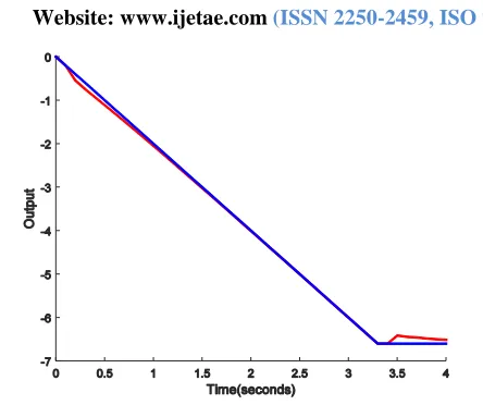
Gain control has been determined after comparing the actual model USV with model predictive based on reference input error reduction and the results achieved for the system states. Finally, the above mentioned two controllers in a cascade controller is located. The overall structure of the controller is shown below. The results of the path to two states is obtained as follows.

Fig. 18. MPC system states

Fig. 19. MPC system states

[image:10.612.69.272.204.562.2]

(11)

International Journal of Emerging Technology and Advanced Engineering

[image:11.612.57.279.121.307.2]

21

Fig. 21. Cascade control system states

IV. CONCLUSION

This paper presented several nonlinear control applications for underactuated nonholonomic systems. An overview of nonlinear control and nonholonomic systems is given and SMC and MPC methods are introduced. A kinematic controller is applied to an experimental wheeled mobile robot for validation of rapid prototyping techniques and new trajectory planning algorithms. The SMCs are developed for setpoint and trajectory tracking of USVs and simulation results are presented. A receding horizon MPC is developed for setpoint and tracking control and simulation examples are given. Finally, a predictive sliding mode cascade controller is developed combining the strengths of the SMC and MPC.

A. Suggestions

1) Mobile Robots

Future work in this area would involve communicating the camera-based position feedback to the mobile robots wirelessly via Bluetooth. A combination of encoder and camera feedback using multi-rate estimation schemes can be employed. This work could also be expanded to include moving obstacles whose position would be determined in real-time by the vision system and transmitted to the mobile robots along with the robots’ absolute positions

2) Cascade Control

In the area of predictive and sliding mode cascade control, future work will include implementation of the proposed techniques on the experimental USV and mobile robot systems.

At the current time, the optimization does not compute quickly enough to implement the controller in real-time. However, the cascade controller parameter sequence may be computed offline and implemented on the experimental system open-loop.

REFERENCES

[1] H. Durrant-Whyte. A Critical Review of the State-of-the-Art in Autonomous Land Vehicle Systems and Technology. Technical report, Sandia National Laboratories, Albuquerque, 2001.

[2] M. Reyhanoglu, A. van der Schaft, N.H. Mcclamroch, and I. K olmanovsky. Dynamics and control of a class of underactuated mechanical systems. IEEE Transactions on Automatic Control, 44(9):1663–1671, 1999.

[3] N.P.I. Aneke. Control of Underactuated Mechanical Systems. PhD thesis, Eindhoven University of Technology, Eindhoven, The Netherlands, 2002.

[4] I. Kolmanovsky and N. H. McClamroch. Developments in nonholonomic control problems. IEEE Control Systems Magazine, 15(6):20–36, 1995.

[5] C. Samson. Time-varying feedback stabilization of car-like wheeled mobile robots. The International Journal of Robotics Research, 12(1):55–64, 1993.

[6] W. Dixon, Z.P. Jiang, and D. Dawson. Global exponential setpoint control of wheeled mobile robots: A lyapunov approach. Automatica, 36:1741–1746, 2000.

[7] A. Z. Anwar, et al. Trajectory Tracking of a Nonholonomic Wheeled Mobile Robot Using Hybrid Controller. International Journal of Modeling and Optimization 6.3 (2016): 136.

[8] Y. Wang, et al. Simultaneous stabilization and tracking of nonholonomic mobile robots: A Lyapunov-based approach. IEEE Transactions on Control Systems Technology 23.4 (2015): 1440-1450.

[9] R. S. Ortigoza, et al. Trajectory tracking control for a differential drive wheeled mobile robot considering the dynamics related to the actuators and power stage. IEEE Latin America Transactions 14.2 (2016): 657-664.

[10] F. Yang, et al. Adaptive and sliding mode tracking control for wheeled mobile robots with unknown visual parameters. Transactions of the Institute of Measurement and Control (2016): 0142331216654534.

[11] A Mazur and M Cholewiński "Implementation of factitious force method for control of 5R manipulator with skid-steering platform REX." Bulletin of the Polish Academy of Sciences Technical Sciences 64.1 (2016): 71-80.

[12] R. Fierro and F. L. Lewis. Control of a nonholonomic mobile robot: Backstepping kinematics into dynamics. Journal of Robotic Systems, 14(3):149–163, 1997.

[13] W. Xie, et al. A simple robust control for global asymptotic position stabilization of underactuated surface vessels. International Journal of Robust and Nonlinear Control (2017).

(12)

International Journal of Emerging Technology and Advanced Engineering

22 [15] L. C. McNinch, H. Ashrafiuon, and K. R. Muske. Sliding mode

setpoint control of an underactuated surface vessel: simulation and experiment. American Control Conference (ACC), 2010. IEEE, 2010.

[16] D. Panagou, and K. J. Kyriakopoulos. Dynamic positioning for an underactuated marine vehicle using hybrid control. International Journal of Control 87.2 (2014): 264-280.

[17] Z. Zhang, and Y. Wu. Switching-based asymptotic stabilisation of underactuated ships with non-diagonal terms in their system matrices. IET Control Theory & Applications 9.6 (2014): 972-980. [18] W. Dong and Y. Guo. Global time-varying stabilization of

underactuated surface vessel. IEEE Transactions on Automatic Control, 50(6):859–864, 2005.

[19] N. Wang, et al. Adaptive robust finite-time trajectory tracking control of fully actuated marine surface vehicles. IEEE Transactions on Control Systems Technology 24.4 (2016): 1454-1462.

[20] P Švec, et al Target following with motion prediction for unmanned surface vehicle operating in cluttered environments. Autonomous Robots 36.4 (2014): 383-405.

[21] J. Ghommam, F. Mnif, and N. Derbel. Global stabilisation and tracking control of underactuated surface vessels. IET control theory & applications 4.1 (2010): 71-88.

[22] Z. Yan, and J. Wang. Model predictive control for tracking of underactuated vessels based on recurrent neural networks. IEEE Journal of Oceanic Engineering 37.4 (2012): 717-726.

[23] A. Thakur, P. Svec, and S. K. Gupta. Generation of state transition models using simulations for unmanned sea surface vehicle trajectory planning. ASME 2011 International Design Engineering Technical Conferences and Computers and Information in Engineering Conference. American Society of Mechanical Engineers, 2011.

[24] C. Liu, Z. J. Zou and J. C. Yin. Path following and stabilization of underactuated surface vessels based on adaptive hierarchical sliding mode. Int. J. Innov. Comput. Inf. Control 10 (2014): 909-918. [25] L. Liu, Z. Liu and J. Zhang. LMI-based model predictive control for

underactuated surface vessels with input constraints. Abstract and Applied Analysis. Vol. 2014. Hindawi Publishing Corporation, 2014.

[26] H. Ashrafiuon, et al. Full state sliding mode trajectory tracking control for general planar vessel models. American Control Conference (ACC), 2015. IEEE, 2015.

[27] H. Ashrafiuon, K. Muske, L. McNinch, and R. Soltan. Sliding-mode tracking control of surface vessels. IEEE Transactions on Industrial Electronics, 55(11):4004–4012, 2008.

[28] L. McNinch, H. Ashrafiuon, and K. Muske. Sliding mode setpoint control of an underactuated surface vessel: Simulation and experiment. 2010 American Control Conference, submitted. [29] L. McNinch, K. Muske, and H. Ashrafiuon. Model-based predictive

control of an unmanned surface vessel. In Proceedings of the 11th IASTED International Conference on Intelligent Systems and Control, pages 385–390, 2008.

[30] L. McNinch, K. Muske, and H. Ashrafiuon. Model predictive control for an autonomous unmanned surface vessel. Control and Intelligent Systems, in press.