Statistical modeling for selecting housekeeper genes

(1)

comm

en

t

re

v

ie

w

s

re

ports

de

p

o

si

te

d r

e

sea

rch

refer

e

d

re

sear

ch

interacti

o

ns

inf

ormation

Statistical modeling for selecting housekeeper genes

Aniko Szabo

*

_{, Charles M Perou}

†

_{, Mehmet Karaca}

†

_{, Laurent Perreard}

‡

_,

John F Quackenbush

§

_{and Philip S Bernard}

‡§

Addresses: *_{Department of Oncological Sciences, Huntsman Cancer Institute, Salt Lake City, UT 84112, USA.}†_{Lineberger Comprehensive}

Cancer Center and Department of Genetics, University of North Carolina, Chapel Hill, NC 27599, USA. ‡_{ARUP Laboratories Inc., Salt Lake City,}

UT 84108, USA. §_{Department of Pathology, University of Utah, Salt Lake City, UT 84112, USA.}

Correspondence: Aniko Szabo. E-mail: [email protected]

© 2004 Szabo et al.; licensee BioMed Central Ltd. This is an Open Access article: verbatim copying and redistribution of this article are permitted in all media for any purpose, provided this notice is preserved along with the article's original URL.

Statistical modeling for selecting housekeeper genes

<p>Genes that exhibit minimal variation in messenger RNA (mRNA) quantity across a variety of cell types and biological conditions pro-vide valuable controls for relative quantification. Normalizing quantitative data with housekeeper genes has many applications, from iden-tifying genes regulated during embryogenesis to developing new cancer diagnostics. Although finding biological significance in gene-expression data can rely heavily on the performance of the housekeeper genes, there is a paucity of information on testing these genes for their suitability for this role.</p>

Abstract

There is a need for statistical methods to identify genes that have minimal variation in expression across a variety of experimental conditions. These 'housekeeper' genes are widely employed as controls for quantification of test genes using gel analysis and real-time RT-PCR. Using real-time quantitative RT-PCR, we analyzed 80 primary breast tumors for variation in expression of six putative housekeeper genes (MRPL19 (mitochondrial ribosomal protein L19), PSMC4 (proteasome (prosome, macropain) 26S subunit, ATPase, 4), SF3A1 (splicing factor 3a, subunit 1, 120 kDa), PUM1

(pumilio homolog 1 (Drosophila)), ACTB (actin, beta) and GAPD (glyceraldehyde-3-phosphate dehydrogenase)). We present appropriate models for selecting the best housekeepers to normalize quantitative data within a given tissue type (for example, breast cancer) and across different types of tissue samples.

Background

Genes that exhibit minimal variation in messenger RNA (mRNA) quantity across a variety of cell types and biological conditions provide valuable controls for relative quantifica-tion. Normalizing quantitative data with housekeeper genes has many applications, from identifying genes regulated dur-ing embryogenesis to developdur-ing new cancer diagnostics. Although finding biological significance in gene-expression data can rely heavily on the performance of the housekeeper genes, there is a paucity of information on testing these genes for their suitability for this role.

The copy number of a housekeeper gene should be propor-tional to the amount of poly(A) RNA present in the sample and this proportion should be maintained across a variety of experimental conditions. As nucleic acids show high

absorb-ance at 260 nm (A₂₆₀), spectrophotometers provide

approxi-mate amounts of total DNA/RNA present in a sample. Using

absorbance methods alone, however, gives no information about the type of nucleic acid (for example DNA versus RNA) or contributions from different nucleic acid fractions (for example rRNA versus mRNA). It is assumed that mRNA com-prises approximately 1-3% of the total RNA. However, this contribution may change depending on the extraction method used. For instance, column extraction methods pro-vide better exclusion of ribosomal RNA than solvent extrac-tion methods [1]. By combining capillary electrophoresis with absorbance, it is possible to accurately quantify these differ-ent fractions [2].

Traditionally, housekeepers have been used in Northern blot analysis to represent the amount of mRNA in the sample and to control for sample loading, blot transfer and probe hybrid-ization. Highly expressed genes serving fundamental roles in the cell are commonly used for this purpose but may not be optimal under certain experimental conditions [3-5]. For

Published: 29 July 2004 Genome Biology 2004, 5:R59

Received: 16 January 2004 Revised: 13 May 2004 Accepted: 11 June 2004 The electronic version of this article is the complete one and can be

(2)

example, the sensitivity and accuracy of northern blot analy-sis with densitometry may be decreased using a highly expressed housekeeper gene that can saturate the autoradio-graphic signal [6]. To resolve this problem and compensate for limitations in dynamic range, control genes may be chosen to have a level of gene expression similar to the gene(s) of interest (that is, the test genes).

Microarrays are more practical for genome-wide expression analysis than northern blots [7]. With cDNA microarrays, a common reference sample is usually used to compare the expression of each gene across many experimental sample(s) [8,9]. Because each gene in the experimental sample is directly compared to the same gene in the common reference, housekeeper genes are not necessary for normalization. Microarrays are commonly applied to finding genes with dif-ferential expression across experimental conditions, however the data may also be used to identify stably expressed genes that can serve as important controls for northern blot analy-sis, ribonuclease protection assays and quantitative reverse transcription PCR (RT-PCR). In turn, these other quantita-tive methods are often used to verify differentially expressed genes identified by microarray [10-12].

Housekeeper genes are often adopted from the literature and used across a variety of experimental conditions, some of which may induce differences in their expression. If unrecog-nized, unexpected changes in housekeeper expression could result in erroneous conclusions about real biological effects such as responses to drugs. In addition, this type of change would be difficult to detect because most experiments only include a single housekeeper gene. It is difficult to determine whether a given gene has the constitutive property of a house-keeper when the true amount of mRNA in a sample is

unknown. As a way round this dilemma, Vandesompele et al.

postulate that gene pairs that have stable expression patterns relative to each other are proper control genes [13]. An alter-native method for quantitative analysis of RT-PCR data that does not require housekeeper genes for normalization is to

use global pattern recognition (GPR). For instance, Akilesh et

al. used a GPR algorithm to search for eligible normalizing

genes within an assay plate and then used those genes as con-trols to identify differentially expressed genes [14].

Although relative quantification using housekeeper genes is a practical method of estimating the expression level of a test gene, the transcript amount in the sample is a summation and the method does not consider transcript differences on a

cell-to-cell basis. Fluorescence in situ hybridization (FISH) is

clin-ically used to determine absolute DNA copy number (for

example, HER2 amplification) in a cell, but these methods

still average the copy number after counting many cells and

the technique is expensive and laborious [15]. In situ methods

for detecting RNA transcripts have been developed but the assays are semiquantitative and subjective [16].

In the work presented here, we applied several models to selecting the best housekeeper genes for breast cancer and give algorithms that can be generalized to find housekeeper genes that are appropriate for normalizing quantitative data within and between tissue types.

Results and discussion

One tissue type

The genes MRPL19, PSMC4, SF3A1, PUM1, ACTB and GAPD

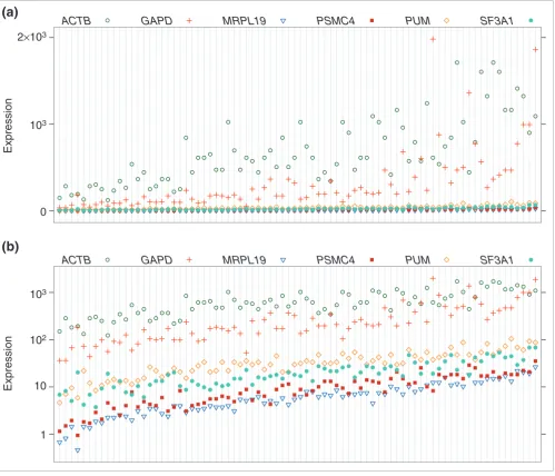
were analyzed by real-time quantitative RT-PCR. Starting copy numbers for the six candidate housekeeping genes were measured across 80 primary breast tumor samples. The data are available as Additional data file 1 with the online version of this article. Plots of the raw and log-scaled expression lev-els (all logarithms in this paper are natural base (e) loga-rithms) are shown in Figure 1. The breast tumor samples are ordered according to the mean of the log-expression levels of all the genes. It is evident from the plot that for the raw data the variability of within-sample measurements increases with the mean expression, whereas the variability stays approxi-mately the same for all the samples with the log-transforma-tion. In addition, the log-transformation allows us to model fold changes in expression levels in an additive way.

To select the best housekeepers for normalizing data across a single tissue type, we tested three variations of a model (Model 1, a-c) with real-time quantitative RT-PCR data gen-erated from primary breast samples (see Materials and meth-ods for details).

Model 1a

We model the expression y_ijof gene j in sample I by

log y_ij= µ+ T_i+ G_j+ ε_ij, where ε_ij~ N(0, )

where µis the overall mean (log-) expression, T_iis the

differ-ence of the ith tissue sample from the overall average and G_j

is the difference of the jth gene from the overall average. The

key feature of this model that makes it different from a tradi-tional ANOVA model is that it allows heteroscedastic errors to account for different variability in the genes [17]. The

varia-bility around the gene-specific mean log-expression µ+ T_i+

G_jis quantified by the error standard deviation σ_j. The

Baye-sian information criterion (BIC) was used to avoid overfitting the data [18]. Model 1a had the best BIC value and was selected from a range of competing models that included a method with equal error variances (Model 1b in Materials and methods) and a more complex method with correlated errors (Model 1c in Materials and methods).

Using Model 1a, standard deviations were determined to select the best control genes for breast cancer. Table 1 shows

that MRPL19 has the smallest variability across the breast

cancer samples and would be the best choice for a single

(3)

comm

en

t

re

v

ie

w

s

re

ports

refer

e

d

re

sear

ch

de

p

o

si

te

d r

e

se

a

rch

interacti

o

ns

inf

o

rmation

housekeeper control. Although some of the confidence inter-vals overlap, a direct comparison between the genes selected

from the microarray (MRPL19, PSMC4, PUM1, SF3A1) to the

classical housekeepers (GAPD and ACTB) shows significant

difference (p = 0.0014).

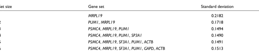
As the biological function of many genes is still unknown, it is difficult to predict how different experimental conditions may affect the expression of putative housekeeper genes. Thus, a safer approach is to use an average expression of several genes that show small variance across conditions. On the basis of the selected model, the estimate of the variance of the log-average of the expression of several genes can be calcu-lated (see Materials and methods for details). Table 2 shows the standard deviations of the log-average of the best gene set

for each possible set size (that is, 1-6). These standard devia-tion values are approximately equal to the coefficient of vari-ation in the original scale. From the estimates, the four-gene

set of PSMC4, MRPL19, PUM1 and SF3A1 provides the lowest

overall variability when choosing a combination of genes. However, this four-gene set is barely different from the

three-gene combination of MRPL19, PUM1 and PSMC4, which in

turn is far better than the best two-gene combination. For

economy, and because SF3A1 had a relatively high individual

variability compared to others in the set, our choice for the normalizing set is the geometric mean of the expressions of

MRPL19, PUM1 and PSMC4.

[image:3.612.57.556.87.515.2]

These findings illustrate the importance of performing an unbiased and genome-wide search for housekeepers rather Relative levels of expression determined by real-time quantitative RT-PCR are shown for 6 housekeeper genes in 80 breast tumors

Figure 1

Relative levels of expression determined by real-time quantitative RT-PCR are shown for 6 housekeeper genes in 80 breast tumors. The top panel displays the raw data and the bottom panel displays a log-scale of the data.

Expression

2×103

103

0

Expression

103

102

10

1

ACTB GAPD MRPL19 PSMC4 PUM SF3A1

(a)

(4)

than relying on traditional housekeeper genes. We used microarray data to select genes with low variability in expres-sion across breast tumors and cell lines. Because the quanti-tative differences between the microarray and RT-PCR platforms are relative, genes with low variability in expres-sion across tumors by microarray should also show low vari-ability in expression by RT-PCR. Although the quantitative data from microarray tends to have an overall smaller dynamic range compared to RT-PCR, this is primarily due to loss of information from genes expressed at low levels. Our microarray dataset was filtered to remove genes with signals near background noise.

The result is very similar using Vandesompele et al.'s M value

method, with only the positions of PUM1 and PSMC4

chang-ing in stability rank. It should be noted that the M-value

method does not order the two best genes (MRPL19 and

PSMC4). Their best gene-set selection approach would sug-gest using the (log-scale) average of these two best genes as a control. Such a concordance is not surprising given the close

relationship between the M value and our model using the

variability of the average of several genes (see Materials and methods for details). A benefit of our approach is the ability to compare the variability of individual genes to that of an average of several genes.

Multiple tissue types

Gene(s) with minimal variation in expression across different cell types serve as good 'universal' housekeepers. A universal control may be a single gene or combination of genes. While the former should display both low variability within a given tissue type and consistent basal levels of expression across tissue types, the latter may comprise a gene set with individ-ually different, but complementary, basal expression levels across tissue types.

To test our models for selecting universal housekeepers, we

used published data from Vandesompele et al. [13]. They

measured the expression level of 10 genes in neuroblastoma cell lines (NB), cultured normal fibroblasts (FIB), normal leu-kocytes (LEU) and cells from normal bone marrow (BM). In addition, normal tissues from pooled organs (breast, brain, fetal brain, heart, kidney, uterus, lung, trachea and small intestine) were also profiled. A plot of these housekeepers across the different tissues is shown in Figure 2. It is notable that a gene can have stable expression within a given tissue type but can change rank position compared to other

house-keepers across tissues. For example, GAPD has relatively high

expression in fibroblasts compared to other housekeepers but

low expression in leukocytes. Thus, GAPD may be a good

[image:4.612.58.555.121.226.2]

single housekeeper within certain tissue types but may not be Table 1

Standard deviation estimates of log expression using Model 1a for selecting the single best housekeeper gene for breast cancer

Gene Estimated standard deviation 95% confidence interval

MRPL19 0.218 (0.168, 0.284)

PUM1 0.265 (0.215, 0.328)

PSMC4 0.288 (0.235, 0.352)

SF3A1 0.393 (0.327, 0.472)

ACTB 0.448 (0.376, 0.533)

GAPD 0.519 (0.439, 0.613)

Table 2

Standard deviation estimates of log expression using Model 1a for selecting the best housekeeper gene(s) for breast cancer

Set size Gene set Standard deviation

1 MRPL19 0.2182

2 PUM1, MRPL19 0.1718

3 PSMC4, MRPL19, PUM1 0.1494

4 PSMC4, MRPL19, PUM1, SP3A1 0.1490

5 PSMC4, MRPL19, SF3A1, PUM1, ACTB 0.1491

[image:4.612.60.554.296.401.2]

(5)

comm

en

t

re

v

ie

w

s

re

ports

refer

e

d

re

sear

ch

de

p

o

si

te

d r

e

sea

rch

interacti

o

ns

inf

ormation

an optimal universal housekeeper unless it is used within a complementary gene set.

Model 2

To compare the performance of housekeepers within and between different tissues, we made a Model 2 (see Materials and methods for further details) that models the expression

of gene j in the ith sample of tissue-type k by

log y_i(k)j= µ+ C_k+ T_i(k)+ G_j+ (CG)_kj+ ε_i(k)j, where ε_i(k)j~

N(0, ))

where µdenotes the overall mean (log-) expression, C_kis the

difference of the kth tissue type from the overall average, T_i₍_k₎

is the specific effect of the ith sample of tissue-type k, G_jis the

difference of the jth gene from the overall average and (CG)_kj

is the tissue-type specific effect of gene j. Variability in

calcu-lation comes from two sources: the specific gene (σ_j) and the

tissue-type (ςk). The estimates of these parameters are given

in Table 3. The single gene with the overall lowest variability

within each tissue type is GAPD, followed closely by UBC

(ubiquitin C), HPRT1 (hypoxanthine

phosphoribosyltrans-ferase 1) and YWHAZ (tyrosine

3-monooxygenase/tryp-tophan 5-monooxygenase activation protein, zeta polypeptide). This result correlates closely with

Vandesom-pele et al.'s approach. That is, the top five genes have exactly

the same order when we rank the genes within each tissue

type according to their M-value. Here we assign a rank of 1.5

to the unordered best pair and then average the ranks to obtain an overall ordering of the genes.

The risk of normalizing data to a housekeeper gene with var-iable overall expression level across different tissues can be represented mathematically as bias error. A housekeeper that has low bias for a particular tissue has an expression level that is near its mean expression across tissues. In our second

model, the term (CG)_kjrepresents this tissue-type specific

bias. The measure of variability around an intended value when bias is present is called the mean squared error (MSE):

MSE = bias2 _{+ variance. Thus, to find a set of genes for}

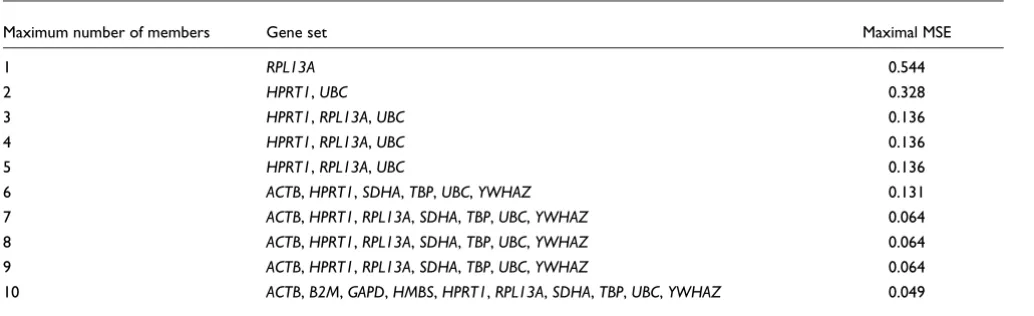
nor-malization across the various tissue types we use a minimax MSE criterion: minimizing the largest MSE of the combina-tion. Table 4 provides a list for the best gene set of each size

along with the minimax-MSE value. Although GAPD has

rel-atively low overall variability within each tissue type, its basal expression changes across tissue types making it a poor choice for a single universal control. The data shows that

RPL13A (ribosomal protein L13a) is the best single universal housekeeper, but it is clear that no single gene is optimal for a universal housekeeper. Actually, choosing all the candidates provides the smallest MSE, which is not surprising as the set of all 10 genes is unbiased by definition. For routine application it is reasonable to limit the number of control Dataset from Vandesompele et al. [13] in log scale-showing expression levels of 10 putative housekeeper genes by sample and tissue type

Figure 2

Dataset from Vandesompele et al. [13] in log-scale showing expression levels of 10 putative housekeeper genes by sample and tissue type. Tissue types analyzed included normal bone marrow (BM), cultured normal fibroblasts (FIB), normal leukocytes (LEU), neuroblastoma cell lines (NB), and pooled normal tissue from breast, brain, fetal brain, heart, kidney, uterus, lung, trachea and small intestine (POOL).

Samples

Expression

BM FIB LEU NB POOL

ACTB

B2M GAPDHMBS HPRT1RPL13A SDHATBP UBCYWHAZ

10−5 10−4 10−3 10−2 10−1 100 101

(6)

genes, as the cost of assaying additional genes needs to balance the extra precision obtained. With this in mind, it is

instructive to note that the three-member set of HPRT1,

RPL13A and UBC is an excellent choice because it maintains a priority ranking even when selection is open to including four- or five-element sets. The housekeeper genes we tested by RT-PCR on breast tumor samples were not assayed across other tissue types and thus could not be evaluated as univer-sal controls. Nevertheless, it is likely that our results in breast tissue would hold up across other tissue types as our genes were initially selected from microarray data that included 17 different and diverse cell lines as well as primary breast tumors [19].

Figure 3 shows the MSE of each gene broken down into the squared-bias and variance components. The direction of each bar shows the sign of the bias. It is apparent that the large bias dominates the large values of MSE. The use of the (log-) average of several genes tends to reduce the variance, due to the effect of bias reduction where opposite biases cancel each

other out. For example, both ACTB and TBP (TATA box

bind-ing protein) have a large bias in the pooled normal samples, but in opposing directions. The mean squared error of the

(log-) average of ACTB and TBP in these samples is only 0.35,

which is much lower than their individual MSEs above 6.

In summary, we have modeled the performance of putative housekeepers to test their goodness-of-fit in serving as normalization controls for relative insert quantification. A major advantage of a model approach is that the terms are

placed within a solid statistical framework and are not ad hoc,

which allows the algorithm to be generalized to a variety of different experimental conditions. The genes and algorithms that we have selected for normalization should have broad utility for diagnostics and research.

Materials and methods

Pre-selection of assayed genes from microarray experiments

Four candidate housekeepers (PSMC4, MRPL19, PUM1 and

[image:6.612.54.565.121.225.2]

SF3A1) were selected from a microarray dataset containing 40 different breast tumors, three normal breast samples and 19 cell lines representing 17 different cell lines of diverse nature including lymphocytes, fibroblasts and epithelial cells [8]. All experiments were done using a common reference Table 3

Components of the standard deviation estimates of the log-expression of the data of Vandesompele et al. [13]

Standard deviation of genes (σ_j)

GAPD UBC HPRT1 YWHAZ SDHA RPL13A TBP HMBS ACTB B2M

0.211 0.226 0.227 0.232 0.255 0.339 0.339 0.431 0.460 0.562

Tissue-type specific multipliers (ςk)

Bone marrow Cultured normal fibroblasts Neuroblastoma cell lines Normal leukocytes Pooled*

1.000 1.204 1.582 1.879 2.014

[image:6.612.56.573.285.443.2]

*Pooled normal tissue from breast, brain, fetal brain, heart, kidney, uterus, lung, trachea and small intestine.

Table 4

Minimax MSE optimal gene sets for each set size

Maximum number of members Gene set Maximal MSE

1 RPL13A 0.544

2 HPRT1, UBC 0.328

3 HPRT1, RPL13A, UBC 0.136

4 HPRT1, RPL13A, UBC 0.136

5 HPRT1, RPL13A, UBC 0.136

6 ACTB, HPRT1, SDHA, TBP, UBC, YWHAZ 0.131

7 ACTB, HPRT1, RPL13A, SDHA, TBP, UBC, YWHAZ 0.064

(7)

comm

en

t

re

v

ie

w

s

re

ports

refer

e

d

re

sear

ch

de

p

o

si

te

d r

e

se

a

rch

interacti

o

ns

inf

o

rmation

strategy in which all experimental samples are compared to the same reference comprised of a pool of RNAs isolated from 11 diverse human cell lines [19].

To select housekeepers, we first 'filtered' the microarray data to select genes with Cy3 and Cy5 signal intensities greater than 500 units across at least 75% of the experiments. This requirement ensures that the gene is well expressed not only in the experimental samples, but also in the common refer-ence sample. Next, we used the SAS/STAT Analysis Package Version 8 (SAS Institute Inc., Cary, NC) to identify a set of genes that showed a small range of expression across sample types and the least variance of the array-mean normalized log-ratios. For real-time RT-PCR, we selected four of the top

six genes - PUM1, PSMC4, MRPL19 and SF3A. The two other

low-variability genes identified in the data were IER3

(imme-diate early response 3) and SRY ((sex determining region

Y)-box 2). We did not select these genes because of their poten-tial for being differenpoten-tially regulated under other conditions.

However, we did include GAPD and ACTB, which are

commonly used reference genes [20], in the set of candidate genes for comparison to the microarray selection.

Samples and cDNA preparation

Breast samples were acquired under informed consent and received at the Huntsman Cancer Institute (Salt Lake City, UT) for gene expression analysis (University of Utah, IRB #8533). All specimens were expediently processed in pathol-ogy upon arrival from surgery. Samples were grossly dissected, procured by flash freezing in liquid nitrogen, and stored at -80°C until RNA extraction. Approximately 50-100 mg cancer tissue was homogenized from each sample, and total RNA was prepared using the RNeasy midi kit (Qiagen). The integrity of RNA was determined using the RNA 6000 Nano LabChip kit (Agilent Technologies) and an Agilent 2100

Bioanalyzer. Two microliters of total RNA (50 ng/µl) were

heated to 70°C and 1 µl was loaded on the column.

Degrada-tion was evaluated using the signal of the 18S and 28S ribos-omal peaks [21].

First-strand cDNA was synthesized from 1 µg total RNA using

[image:7.612.54.554.86.379.2]

oligo(dT) primers and Superscript III reverse transcriptase following manufacturer's instructions (Superscript III First-Strand Synthesis System, Invitrogen Life Technologies). Briefly, the reaction was held at 48°C for 50 min, followed by Mean squared error (MSE) of each gene by tissue-type

Figure 3

Mean squared error (MSE) of each gene by tissue-type. The sign is determined by the direction of the bias. The MSE is broken down into the contributing components of the squared bias (Bias2_{) and the variance (Sigma}2_{). Dataset from Vandesompele}_{et al}_{. [13]. Tissue types analyzed included normal bone}

marrow (BM), cultured normal fibroblasts (FIB), normal leukocytes (LEU), neuroblastoma cell lines (NB), and pooled normal tissue from breast, brain, fetal brain, heart, kidney, uterus, lung, trachea and small intestine (POOL).

Signed MSE

ACTB B2M GAPD HMBS HPRT1

RPL13A SDHA TBP UBC YWHAZ

Bias2 _Sigma2

BM FIB _LEU NB

POOL

BM FIB _LEU NB

POOL

BM FIB _LEU NB

POOL

BM FIB _LEU NB

POOL

BM FIB _LEU NB

POOL

−5 0 5

(8)

a 15 min step at 70°C. The cDNA was washed on QIAquick

PCR purification column (Qiagen) and eluted in 2 × 50 µl of

elution buffer. The cDNA was then diluted in TE' (10 mM Tris, 0.1 mM EDTA, pH 8.0), aliquoted and stored at -80°C for fur-ther use.

Real-time quantitative PCR

All PCR reactions were performed on the LightCycler. Each

20 µl reaction included 1 × PCR buffer with 3 mM MgCl₂

(Idaho Technology), 0.2 mM each of dATP, dCTP, and dGTP (Roche), 0.1 mM dTTP (Roche), 0.3 mM dUTP (Roche), 1 U of Platinum taq (Invitrogen Life Technologies), 1/40000 SYBR Green I (Molecular Probes), approximately 5 ng cDNA,

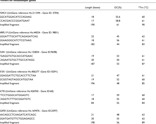
and 0.4 µM of each primer. The primers used for the RNA

control genes are shown in Table 5.

[image:8.612.60.558.273.669.2]

PCR was done using the following protocol: initial denatura-tion 95°C for 1 min 30 sec, then 50 cycles at 94°C for 1 sec for denaturation, 60°C for 5 sec (20°C/sec transition) for anneal-ing, 72°C for 8 sec (2°C/sec transition) for extension. Fluores-cence emission of SYBR Green I (channel 1, 530 nm) was acquired each cycle after the extension step. A melting step was performed after PCR to determine product purity. For melting curve analysis, the reactions were rapidly (20°C/sec) cooled from 95°C to 60°C and then slowly heated (0.1°C/sec) back to 95°C while continuously monitoring fluorescence.

Table 5

Primers for housekeeper genes

Length (bases) GC(%) *Tm (°C)

PSMC4 (UniGene reference Hs.211594 - Gene ID: 5704)

GGCATGGACATCCAGAAG 18 55.6 60

CCACGACCCGGATGAAT 17 58.8 61

Amplified fragment 190 61 90

MRPL19 (UniGene reference Hs.44024 - Gene ID: 9801)

GGGATTTGCATTCAGAGATCAG 22 45 62

GGAAGGGCATCTCGTAAG 18 56 61

PUM1 (UniGene reference Hs.153834 - Gene ID:9698)

TGAGGTGTGCACCATGAAC 19 53 61

CAGAATGTGCTTGCCATAGG 20 50 61

SF3A1 (UniGene reference Hs.406277 -Gene ID:10291)

GGAGGATTCTGCACCTTCTAA 21 47 61

GCGGTAGTAGGCATGGTAA 19 52 60

ACTB (UniGene reference Hs.426930 - Gene ID:60)

TTCCTGGGCATGGAGTC 17 59 60

CAGGTCTTTGCGGATGTC 18 55 60

†_GAPD_{(UniGene reference Hs.169476 - Gene ID:2597)}

AACAGCCTCAAGATCATCAGC 21 48 63

GGATGATGTTCTGGAGAGCC 20 55 62

*Primers Tm determined using Tm Utility with algorithms adapted from Santa Lucia [23]. The Tm for the amplified fragment is the empirical Tm.

(9)

comm en t re v ie w s re ports refer e e d re sear ch de p o si te d r e sea rch interacti o ns inf ormation Relative quantification

Copy number was determined using the crossing point (Cp) value, which is automatically calculated using the LightCycler 3.5 software (Roche Molecular Biochemicals). The Cp value is reported as a fractional cycle number that is determined from the second derivative maximum (point of maximum acceler-ation) on the PCR amplification curve (fluorescence versus cycle number) [22]. A relative starting copy number was determined for each housekeeper using a calibration curve

done with the same batch of master mix. Efficiency (E) of PCR

was calculated from a plot of Cp versus log ng cDNA [22].

E = 10-1/slope

Modeling expression data

As the effects of interest are fold changes, we modeled the log-transformed expression Model 1a.

log y_ij= µ+ T_i+ G_j+ ε_ij,

where independent

where µdenotes the overall mean (log) expression, T_iis the

difference of the ith tissue sample from the overall average

and G_jis the difference of the jth gene from the overall

aver-age. The key feature of this model that makes it different from a traditional ANOVA model is that it allows heteroscedastic errors: the variability of the genes is different.

We fitted the model using the gls routine of the nlme library for R, however other commonly available software such as PROC MIXED from SAS could have been used.

Based on the model, the variability of the logarithm of the geometric mean

of a gene-set S was estimated as

Vandesompele et al.'s M-value is the average of relative

standard deviations of the log-expression levels. Under

Model 1, the M-value of the gene is closely related to its

vari-ance (under Models 2 and 3 below, the similar relationships can be derived):

We tested the assumption of unequal variances by fitting Model 1b that forces all the genes to have the same variability (this is the classical ANOVA model).

log y_ij= µ+ T_i+ G_j+ ε_ij,

where independent

Model 1c with a correlated error structure can be used to assess the assumption of (conditional) independence of the genes given the sample mean. If warranted, a more compli-cated correlation structure can be imposed.

log y_ij= µ+ T_i+ G_j+ ε_ij,

where

For the multiple tissue-type set-up the notation and the model need to be extended. We will denote the expression

level of gene j of in the ith sample of type k by y_i₍_k₎_j, i = 1,...n_k,

j = 1,...,g and k = 1,...,m. The best-fitting model for the data,

which we call Model 2, had the form

log y_i(k)j= µ+ C_k+ T_i(k)+ G_j+ (CG)_kj+ ε_i(k)j,

where

Thus the errors are independent and their variability is decomposed into a gene-specific and tissue-type specific mul-tiplicative components. The last restriction ensures the uniqueness of the solution. Simpler models that we consid-ered used uniform error variance, equal error variance for tis-sue types, and equal error variance for genes. We also considered more complex models that used exchangeable correlation structure for the errors and unstructured error variance (each gene-tissue-type combination has a variance parameter). The BIC was used as a basis for model selection.

Additional data files

Additional data available with this paper online is an Excel file with the relative copy numbers of six genes in the 80 breast cancer samples used in this study (Additional data file 1).

Additional data file 1

An Excel file with the relative copy numbers of six genes in the 80 breast cancer samples used in this study

Click here for additional data file

T_i G N

i n j j g ij j = =

∑

₁ =0,

∑

₁ =0,ε ∼

( )

0,σ2

y_iS ₌ _{j S}y_ij S

∈

∏

( )1/

Var

(

log Var og y_iS

)

=

∑

_{j S}_∈

(

l y_ij

)

/ S =

∑

_{j S}_∈ σ2_j/ S.

V_jk SD y_ij y_ik SD y y

i n ij ik i n = 

{

(

)

}

     = 

{

( )

−

( )

}

 = =

log / log log

1  1

   = + =

(

−

)

= + − ≠ =

∑

≠

σj k

j jk j

k j

k j

k g

M V g

g k j 2 2 2 2 2 1 1 1 1 σ

σ σ σ

/ /

,...,

σσj j σj σ σ

i k k i

R M R R

2 _{1 1}₊ _/ 2_≤ _≤ 2 ₁₊ 2_, ₌_max _/ ,

where

T_i G N

i n j ij j g = =

∑

₁ =0,

∑

₁ =0,ε ∼

( )

0,σ2

T_i G N

i n

j i ig

j g g = =

∑

=

∑

= =

(

)

′

(

)

=

(

)

1 1 1

1

0 0

1

, ,εε_i ε ,...,ε ,

σ σ

ρ

∼ 0 ∑

∑ and ρ ρ ρ ρ ρ σ σ 1 1 1                       . g

C_k T G CG CG

k m i k i n j j g j g

kj k kj

m k

= = ( ) = = =

∑ ₁ =0,∑ ₁ =0,∑ ₁ =0,∑ ₁( ) =∑ ₁( ) =00

0 2 2 1

1

,

, .

(10)

Acknowledgements

This work has been supported in part by the National Cancer Institute (R33 CA097769-01).

References

1. Miller CL, Yolken RH: Methods to optimize the generation of cDNA from postmortem human brain tissue.Brain Res Brain Res Protoc 2003, 10:156-167.

2. Panaro NJ, Yuen PK, Sakazume T, Fortina P, Kricka LJ, Wilding P: Evaluation of DNA fragment sizing and quantification by the Agilent 2100 bioanalyzer.Clin Chem 2000, 46:1851-1853. 3. Suzuki T, Higgins PJ, Crawford DR: Control selection for RNA

quantitation.Biotechniques 2000, 29:332-337.

4. Bhatia P, Taylor WR, Greenberg AH, Wright JA: Comparison of glyceraldehyde-3-phosphate dehydrogenase and 28S-ribos-omal RNA gene expression as RNA loading controls for northern blot analysis of cell lines of varying malignant potential.Anal Biochem 1994, 216:223-226.

5. Spanakis E: Problems related to the interpretation of autora-diographic data on gene expression using common constitu-tive transcripts as controls.Nucleic Acids Res 1993, 21:3809-3819. 6. Eggert A, Brodeur GM, Ikegaki N: Relative quantitative RT-PCR protocol for TrkB expression in neuroblastoma using GAPD as an internal control.Biotechniques 2000, 28:681-691.

7. Schena M, Shalon D, Davis RW, Brown PO: Quantitative monitor-ing of gene expression patterns with a complementary DNA microarray.Science 1995, 270:467-470.

8. Perou CM, Sorlie T, Eisen MB, van de Rijn M, Jeffrey SS, Rees CA, Pol-lack JR, Ross DT, Johnsen H, Akslen LA, et al.: Molecular portraits of human breast tumours.Nature 2000, 406:747-752.

9. van de Vijver MJ, He YD, van't Veer LJ, Dai H, Hart AA, Voskuil DW, Schreiber GJ, Peterse JL, Roberts C, Marton MJ, et al.: A gene-expression signature as a predictor of survival in breast cancer.N Engl J Med 2002, 347:1999-2009.

10. Dhanasekaran SM, Barrette TR, Ghosh D, Shah R, Varambally S, Kura-chi K, Pienta KJ, Rubin MA, Chinnaiyan AM: Delineation of prog-nostic biomarkers in prostate cancer. Nature 2001, 412:822-826.

11. Welsh JB, Zarrinkar PP, Sapinoso LM, Kern SG, Behling CA, Monk BJ, Lockhart DJ, Burger RA, Hampton GM: Analysis of gene expres-sion profiles in normal and neoplastic ovarian tissue samples identifies candidate molecular markers of epithelial ovarian cancer.Proc Natl Acad Sci USA 2001, 98:1176-1181.

12. Mischel PS, Nelson SF, Cloughesy TF: Molecular analysis of gliob-lastoma: pathway profiling and its implications for patient therapy.Cancer Biol Ther 2003, 2:242-247.

13. Vandesompele J, De Preter K, Pattyn F, Poppe B, Van Roy N, De Paepe A, Speleman F: Accurate normalization of real-time quantitative RT-PCR data by geometric averaging of multi-ple internal control genes. Genome Biol 2002, 3:research0034.1-0034.11.

14. Akilesh S, Shaffer DJ, Roopenian D: Customized molecular phe-notyping by quantitative gene expression and pattern recog-nition analysis.Genome Res 2003, 13:1719-1727.

15. Tubbs RR, Pettay JD, Roche PC, Stoler MH, Jenkins RB, Grogan TM: Discrepancies in clinical laboratory testing of eligibility for trastuzumab therapy: apparent immunohistochemical false-positives do not get the message. J Clin Oncol 2001, 19:2714-2721.

16. Kristt D, Turner I, Koren R, Ramadan E, Gal R: Overexpression of cyclin D1 mRNA in colorectal carcinomas and relationship to clinicopathological features: an in situ hybridization analysis.Pathol Oncol Res 2000, 6:65-70.

17. Pinheiro JCBD: Mixed-effects Models in S and S-PLUS New York: Springer; 2000.

18. Schwarz G: Estimating the dimension of a model. Annls Stat 1978, 6:461-464.

19. Perou CM, Brown PO, Botstein D: Tumor classification using gene expression patterns from DNA microarrays.New Tech-nologies for Life Sciences: A Trends Guide 2000:67-76.

20. Roux S, Pichaud F, Quinn J, Lalande A, Morieux C, Jullienne A, de Ver-nejoul MC: Effects of prostaglandins on human hematopoietic osteoclast precursors.Endocrinology 1997, 138:1476-1482. 21. Frank SG, Bernard PS: Profiling breast cancer using real-time

quantitative PCR. In Rapid Cycle Real-Time PCR: Methods and

Appli-cations Edited by: Wittwer CT, Meuer S, Nakagawara K. Heidelberg: Springer; 2003:95-106.

22. Rasmussen RP: Quantification on the LightCycler. In Rapid Cycle Real-Time PCR: Methods and Applications Edited by: Wittwer CT, Meuer S, Nakagawara K. Heidelberg: Springer; 2003:21-34. 23. SantaLucia J: A unified view of polymer, dumbbell, and