Edge Detection With Multi-Scale Undecimated Discrete Wavelet Transform

International Journal of Emerging Technology and Advanced Engineering

159

Edge Detection With Multi-Scale Undecimated Discrete

Wavelet Transform

Fatma ZRIBI

, Professeur Noureddine ELLOUZE

1,2 _{Université de Tunis El Manar, Unité de Recherche Signal Image et Reconnaissance de Formes, ENIT, Tunis, TUNISIE}

Abstract— This paper presents an approach of edge detection by multi-scale undecimated discrete wavelet transform. Haar wavelet is used for this detection which models the theorical representation of an edge. The advantage of this approach is the combination between filtering step and detection one. To consolidate the result of our method we present a measure of edge localization’s by calculating distance from a real square edge’s and the detection’s result of our approach compared to canny detector’s result.

Keywords— mutil-scale edge detection; undecimated wavelet transform.

I. INTRODUCTION

Wavelets are mostly used in image processing for enhancement, filtering and edge detection [1]. Edge detection in occupied a large of interest of computer vision to extract image characterization, to quantify measurement or for recognition process. The wavelet analysis was introduced in the early 80s in the context of signal analysis and oil exploration [2]. It was, at the time, to give a representation of the signals for the simultaneous development time and frequency information (time-frequency location). In 1984, P. Goupillaud , A. J. Grossmann and Morlet [2], pushed by the increasing demands of hydrocarbon research, propose a method for reconstructing multidimensional seismic signals to restore

high frequencies using representation of a "time- frequency ".

II. WAVELET TRANSFORMATION ANALYSIS

To analyze the transient components of different lengths, it is necessary to use atoms whose temporal supports have variable sizes. For this wavelet transform decomposes the signals on a translated and dilated wavelet family. A wavelet is a function that has an average of zero:

  

It is normalized to ‖Ψ‖=1, and centered in the

neighborhood of t = 0. A family of atoms "time-frequency"

is produced by dilating the wavelet Ψ by a factor a, and by

translating it by b: (equation 2)

         a b t a t b a 1 ) ( ,



These atoms still have the norm of 1: ‖Ψ_ (a,b) = 1 ‖ .

The wavelet transform of f∈L ^ 2 (R) at time μ and scale s

for a 1D signal is: (equation 3)

dt a b t a t f b a f s u Wf           

_

Where W is the initial Wavelet [3].

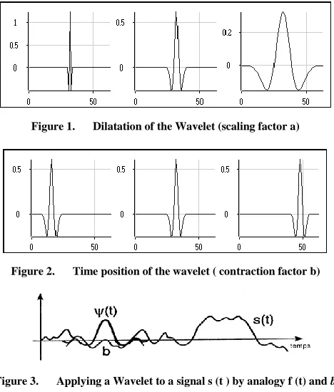
To take consideration of the high and low frequencies, we will simply contract or dilate the reference wavelet Ψ(t). The example below shows one of the wavelet (Wavelet Mexican Hat), with different expansion factors: (figure 1 and figure 2)

Figure 1. Dilatation of the Wavelet (scaling factor a)

Figure 2. Time position of the wavelet ( contraction factor b)

Figure 3. Applying a Wavelet to a signal s (t ) by analogy f (t) and b

International Journal of Emerging Technology and Advanced Engineering

160 The analysis is performed by means of a function specific analysis Ψ called base Wavelet. During the scan, this Wavelet is positioned in the time domain to select the part of the signal to be processed. Then, it is expanded or contracted by using a scaling factor to focus the analysis on a given range of oscillation. When the wavelet is dilated, the analysis looks at the components of the signal that oscillates slowly; when it is contracted, analysis observes the rapid oscillations like contained in a signal discontinuity (Figure3).

With this scaling, the Wavelet transform decomposition leads to a time signal [4].

A. Some examples of Wavelets

We will give some examples of analysis Wavelet (mother) and some properties.

 Continuous Wavelet (Mexican Hat)

The Mexican hat real wavelet that takes its name from its shape, is built from the second derivative of the Gaussian:

) 2 1 exp( ) 1

( 2 2

)

(

t

CM  



(4)

Figure 4. (a) Wavelet, (b) Fourrier transform

This wavelet is symmetrical, which allows not to introduce shifts (phase shifts) in the wavelet transform. Unlike antisymmetric wavelet, (like compact support orthogonal Daubechies wavelets), which it is particularly suitable for the detection of discontinuities.

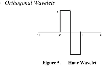
 Orthogonal Wavelets

Figure 5. Haar Wavelet

This wavelet is known since the early 20th century, at the time we were looking for simple orthonormal bases of L^2 (R) and the Haar Wavelet provides an example simply (Figure 5):

(5)

We have used theoretically this Wavelet for our system of edge detection. (equation 5)

This wavelet has the disadvantage of being non-continuous.

The second orthogonal Wavelet is the Daubechies one (Figure 6):

Figure 6. Daubechies Wavelet

For value r, Ingrid Daubechies (1990) completed the work Haar in 1987., Daubechies built an orthonormal base L ^ 2 (R) of the form: (equation 6)









K

j

K

X

,

)

2

(

2

Indeed, Ψ is defined on a compact support (we like to clarify that in general, compactly supported wavelets have no analytical form in particular, Daubechies wavelets have no analytical form. We know how to calculate the function, but cannot express it with a formula) [0; 2r + 1] and satisfies the equation : (equation 7)













X

dX

X

X

dX

r

(

)

(

)

(7)

Where Ψr(x) has r continuous derivatives. When r = 0, Ψr(x) is set to [0; 1], we fall back on the Haar system. In practice we utlise the db1 wavelet Daubechies grade 1 to model the Haar wavelet.

B. Wavelet two-dimensional Discrete Transform

Set of wavelets derived from a reference Wavelet by dilation and translation operations. The user can choose his games Factors of expansion and free way offsets.

International Journal of Emerging Technology and Advanced Engineering

161 The Discrete Wavelet Transform (DWT) from this account to achieve a particularly efficient algorithm, which can easily be intuitively understood.

The basic principle of the DWT. is to separate the signal into two components, one representing the general shape of the signal, the other representing its details. The general appearance of a function is shown by its low frequency and the details of its high frequencies.

To separate the two, so we need a pair of filters: a low pass filter to get the general shape (also called approximation or average) and a high pass filter to estimate its details, which are ie the elements that very quickly. To avoid losing information, these filters must of course be complementary: the frequencies cut by one shall be kept by the other. It is said that the two filters form a pair of quadrature mirror filters (Figure7) [5].

Figure 7. Decomposition of a signal with decimation

Where the symbol represents the sub-sampling or

decimation operation: we take a point signal on both. Each pair of quadrature filters is associated to a wavelet Ψ (t) and a scale function Ψ(t). The Wavelet is an oscillating function for reporting the details of the signal. The scaling function is a low frequency function, associated with the approximation of the signal.

The image, as we know, is a 2D two-dimensional signal, the extension to the 2D is generally performed using a 1D filter product. In practice, the transformation is calculated by applying a bank of separable filters in the image (Figure 8):

Figure 8. Wavelet decomposition with decimation ( we interested only the first portion of the diagram )

In the case of an image signal, the idea is simple, as any filter applied to an image, simply multiply the coefficients of the wavelet (after discretisation) by the value of pixels of the image that will be treated . We note that the wavelet can then be represented in the form of a table (of size 1) of decimal value. In reality, it existing two tables of the coefficients of the Wavelet because it consists of two filters: a low-pass and high-pass [6].

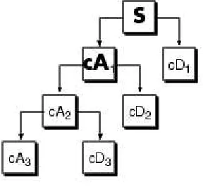
C. Multiresolution Wavelet Decomposition Analysis

A pair of complementary filters low passes and high passes one. Each other, turns a signal length of N into two signals of length N/2: one representing the trend of the signal and called approximation, the other represent details. We say that we spent at a lower resolution.

The approximation is a smoothed version of the start signal, but it still contains noise. Nothing prevents us from repeating the filtering operation on the approximation signal, to access an even lower resolution, and so on.

We can represent this algorithm in the following diagram (Figure 9):

International Journal of Emerging Technology and Advanced Engineering

162 For DWT only the approximation signals are again decomposed. Details of signals from the high-pass filtering are not changed with every step.

At each iteration, we divide the resolution by 2. That's why this method is called multi-resolution analysis. We stop when we reach the desired resolution or when the decomposition is not possible. Therefore, the signal is broken into components of low resolution. The number of iterations performed is called decomposition level.

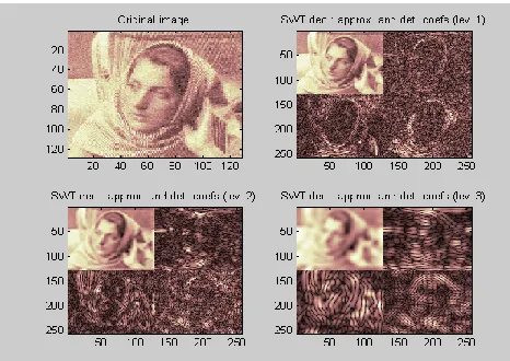
Here we present an example of multiresolution wavelet decomposition of the original image "Woman" from the SWT2 function in Matlab (Figure10):

Figure 10. Women decomposition image in 3 levels with SWT2 of Matlab

D. Discrete Wavelet Transform Redundant

a) Undecimated Wavelet Transform:

The dyadic wavelet transforms are scale sampling wavelet transforms following a geometric progression of reason 2. The time is not sampled.

This transform uses dyadic wavelet.

The dyadic wavelet transform of f is defined by [1] (equation 8)

(8)

With (9)

Indeed this transform algorithm uses a hole that create redundancy information for maintaining invariance in translation at all levels of decomposition. In addition, it provides good spatial location of the lower frequencies as shown in the following scheme (Figure 11):

Figure 11. Decomposition algorithm of the image a by the Redundant Wavelet Transform

Wavelets are tools in signal processing and image simultaneously integrating location and scale parameters.

It exists two types of transformed Wavelet: continuous and discrete.

The work done by these two transforms are different in the field of imaging:

 Continuous Wavelet Transform is known as an

innovative technique in detecting contours of medical images where has proven its relevance. Examples include: outline detections on two radios dry vertebrae, application to 3D reconstruction [7].

 The Discrete Wavelet Transform (DWT) is a

technique used in the compression of digital data with or without loss (JPEG2000). Compression is achieved by successive approximations of the initial information from the coarsest to finest. Then we reduce the size of the information by choosing a level of detail.

In our work, we applied the Discrete Wavelet Transform (DWT), using the dyadic transformation on different test images’ and real images to detect their contours.

III. EDGE DETECTION BY MULTI-SCALE UNDECIMATED

DISCRETE WAVELET TRANSFORM

The performance of a detector is closely related to its calculation time and its efficiency of detection. The effectiveness of detectors can be defined according to the following three criteria (Canny, 1986):

 Good detection: all contours must be detected (without

omission of pixels on the contour which will be detected )

 Good location: the detected contours must be in their

ideal position.

 Elimination of multiple responses: a detector does not

International Journal of Emerging Technology and Advanced Engineering

163 For this there are many edge detection algorithms such as DWT, which was used during a great period for edge detection and more specifically the singularities of an image [8].

This algorithm is based on edge detection by the multi-scale method derived from a Discrete Wavelet Transform without Decimation. The use of the transform without decimation improves the location of the detected edges [9]. Our algorithm was inspired by the work of Michael Weeks and Evelyn Brannock [1] and is given by the diagram below:

Figure 12. Edge detection with multiscale Undecimated Wavelet Transform Algorithm

The algorithm of edge detection with Multi-Scale Undecimated Wavelet Transform (MSUWT) is composed of five steps (Figure 12). The first step is the decomposition of the initial image into three levels which give for each level four image of coefficients. The first image is composed of the image approximation resulting from the low pass filter and three images of details coefficients: vertical, horizontal and diagonal one. The next step is the multi-scale product of each of the three levels. The third step is the calculation of the image contour given by the norm of the product result of the three levels. The fourth step is the thresholding of the image edges with the hysteresis algorithm. Finally we obtain the edge image with the elimination of noise by using the multi-scale product which is the characteristic of this approach.

IV. EXPERIMENTAL RESULTS

The type of the analysing Wavelet is crutial to treat the specific problematic. Indeed for detection edges, we have choose the Debechies db1 Wavelet which modelise the first derivative function of a gaussien as the classical first derivative degree. This Wavelet has a nul moment which approve the modelisation of the first degree of a step edge

We have realised tests to prouve that contour detection with Undecimated Discrete Wavelet Transform is better that the classical detectors. To do these test we have created a test square image where we know exactly the resulting image edges and we have realised these tests:

Figure 13. Left: result of MSUWT. Middle: Ideal Contour. Right:Canny detection result

Figure 14. Thresholding with Hysterisis Algorithm. Left: Our approach MSUWT results. Middle: Ideal contour. Right: Canny

results.

Figure 15. Threshoding with Otsu Algorithm. Left: Our approach MSUWT results contour. Middle: Ideal contour. Right: Canny results

contour

International Journal of Emerging Technology and Advanced Engineering

164

Figure 16. (Left) application of the MSUWT to Lena image. (Right) application of the Canny detector to Lena image

Table 1 present a comparaison of the distance between the each pixels detected with the two algorithms MSUWT and Canny one compared to the ideal contours of the squere. The results gived by this table is the mean distance between each pixel and his corresponded one on the ideal contours of the square. For the Canny detector the means distance is about 0.21 pixels. But for the MSUWT with hysterisis threshoding is about 0.07 pixels and for MSUWT with Otsu thresholding is 0.1 pixels.

TABLE1

. Canny db1 with

hytérisis

db1 with

Otsu

Distance 0.2131 0.0794 0.1004

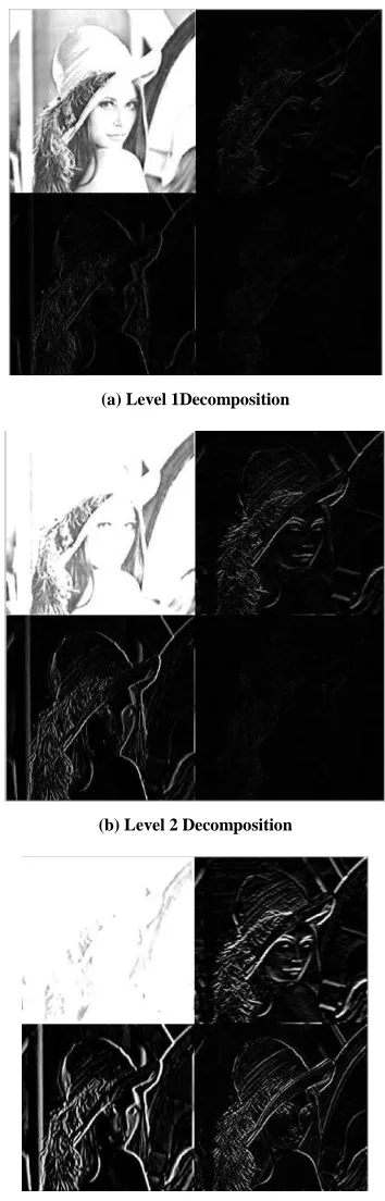
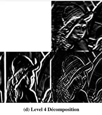
To achieve this result we have varied levels of decomposition between 2 and 4 levels to ensure the selection of the best one. Indeed starting from the theory, if we have a larger number of decomposition levels we will win more details. For this, we tried to vary the scales. The figure below shows the different levels as well as the test results:

(a) Level 1Decomposition

(b) Level 2 Decomposition

International Journal of Emerging Technology and Advanced Engineering

165

(d) Level 4 Décomposition

Figure 17. Edge detection : « Lena » Image decomposed in 4 different levels

After application of our algorithm we obtained these results:

Figure 18. Edge obtained with different level of the MSUWT. Left: 2 levels. Middle: 3 levels. Right: 4 levels.

According to the figures of Figure 18 we conclude that the decomposition into 3 levels is the best to get the maximum detail, since the level 4 has not brought improvement from the level 3 but we note that on the contrary it gives less information than the level 4, 2 or 1. (Figure 17)

V. CONCLUSION

In this paper, we presented the edge detection algorithm

with Multi-Scale Undecimated Wavelet Transform

(MSUWT).

The algorithm is based on multi-scale product for extracting, by an effect of zoom and fine scales, image details, which are the direct result of the wavelet decomposition, for better detection and localization contours of the image.

We presented the different experimental tests of the algorithm for which we have achieved satisfying results. These tests consist in an analysis of the location of the pixels contours in comparison with the Canny edge detector. The results show that the detector has developed a better localization of the pixels contours at the corners of a square compared to the Canny edge detector.

Experimentally the better combination of the levels of the decomposition is three ones. These three decompositions will be used for the multi-scale product avoiding the noise reduction.

REFERENCES

[1] S. Mallat, A Wavelet Tour in Signal Processing, Elsevier, 2009 [2] J.C. Barriere, “Les ondelettes appliquées à l’analyse des signaux

géomagnétiques, examen probatoire”, thesis, 2000, pp.4.

[3] O. Le Cadet, “Méthodes d’ondelettes pour la segmentation d’images. Application à l’imagerie médicale et au tatouage d’images”, thesis, Chapter I la transformée en ondelette continue,

[4] J. Dumas, 01dB-STELL (Group MVI technologies), L’analyse temps-fréquence, February 2001, pp6.

[5] Library Wavelets Version 1.0, “Bibliothèque Ondelettes for MUSTIG”, Chapter 2 Transformée en ondelettes discrete, pp 23. [6] mini project report, “Traitement des images par les ondelettes”,

2005.

[7] V. Kitanovski, D. Taskovski, L. Panovski , Multi-scale Edge Detection Using Undecimated Wavelet Transform, Department of Electronics, FEIT, University Ss Cyril and Methodius, 2008 [8] V. Perrier, “Application de la théorie des ondelettes”, Laboratoiry of

Modelisation and Calculation of IMAG National Institute of Polytechnics of Grenoble, 4-18 march 2005.

[9] S. Mallat, Une exloration des signaux en ondelettes par une introduction aux ondelettes adaptées par le Web, http://cas.ensmp.fr/~chaplais/Wavetour_presentation/Wavetour_pres entation_fr.html#fra