Munich Personal RePEc Archive
A universal solution for units-invariance
in data envelopment analysis
Xu, Jin and Zervopoulos, Panagiotis and Qian, Zhenhua and
Cheng, Gang
29 September 2012
Online at
https://mpra.ub.uni-muenchen.de/41633/
1
A universal solution for units-invariance in data envelopment analysis
Jin Xu
China Center for Health Development Studies, Peking University, 38 Xueyuan Rd, Beijing, China
Panagiotis D. Zervopoulos
China Center for Health Development Studies, Peking University, 38 Xueyuan Rd, Beijing, China
Department of Business Administration of Food and Agricultural Enterprises, University of Ioannina, 2 Georgiou Seferi St, Agrinio, Greece
Zhenhua Qian
School of Social Science, University of Science and Technology Beijing, 30 Xueyuan Rd, Beijing, China
Gang Cheng*
China Center for Health Development Studies, Peking University, 38 Xueyuan Rd, Beijing, China
*Corresponding author
Abstract: The directional distance function model is a generalization of the radial model in data envelopment analysis (DEA). The directional distance function model is appropriate for dealing with cases where undesirable outputs exist. However, it is not a units-invariant measure of efficiency, which limits its accuracy. In this paper, we develop a data normalization method for DEA, which is a universal solution for the problem of units-invariance in DEA. The efficiency scores remain unchanged when the original data are replaced with the normalized data in the existing units-invariant DEA models, including the radial and slack-based measure models, i.e., the data normalization method is compatible with the radial and slack-based measure models. Based on normalized data, a units-invariant efficiency measure for the directional distance function model is defined.
Keywords: Data Envelopment Analysis; Data normalization; Units-invariance; Directional distance function
1. Introduction
2
which means that efficiency scores assigned to DMUs are independent of the measurement units of the inputs and outputs that are utilized in the assessment process (Lovell & Pastor, 1995; Tone, 2001). Radial DEA models, such as CCR and BBC models (Banker et al., 1984; Charnes, 1994), and the radial measure, such as the slack-based measure (SBM), are units-invariant (Färe & Knox Lovell, 1978; Tone, 2001 ).
The directional distance function model is a generalization of radial models (Chambers et al., 1996; Chambers et al., 1998; Chung et al., 1997). A special feature of the directional distance function model is that the direction the DMUs under evaluation are projected to the production frontier can be customized. By assigning a direction vector in Euclidean space, one can project the evaluated DMU on a specific point on the frontier. Particularly when the direction vector points towards the origin of the coordinates, the directional distance function model is equivalent to the radial model. Two advantages of the directional distance function model are that: 1) researchers can specify the direction of decreasing inputs and increasing outputs by assigning a direction vector, and 2) researchers can easily deal with the cases where undesirable outputs exist. However, a drawback of the directional distance function is that its measurement is generally not units-invariant. Taking into account that the inputs and outputs of the evaluated DMUs serve as the direction vector, changes in the measurement units of inputs or outputs potentially can lead to significant differences in the results.
The proposed data normalization method provides a universal solution when the applied DEA model violates the units-invariance criterion. The properties of the proposed method are tested with the DEA-based directional distance function model, but the new method can be applied to all existing and future DEA models.
2. The method of data normalization of DEA and its properties
The measurement of efficiency using radial DEA models is not affected by the measurement units of inputs and outputs because efficiency results from the comparison of the inputs and outputs of the evaluated DMU against the corresponding values of the target DMU (benchmark). For radial models, the inputs or outputs are improved in proportion. In non-radial models, such as SBM models, the “proportional improvement” restriction is loosened, but the measurement of efficiency still draws on input-output ratios. As a result, efficiency scores are not affected by the measurement units of inputs and outputs.
The concept used to develop a method for dealing with the issue of units-invariance is based on the introduction of a preparation stage prior to the application of DEA models. In this stage, the original input and output data are converted into dimensionless data. When dimensionless data are utilized, this stage ensures that the efficiency scores produced by any DEA model will meet the units-invariance criterion.
The proposed procedure is expected to satisfy the conditions below:
3
(2) The results produced by DEA models using converted data can be converted reversely so that to be completely consistent with the results obtained from DEA models utilizing original data. The consistency of the results should be expected regardless of the units-invariance DEA model (i.e., radial or non-radial) that is applied.
The above two conditions ensure the proposed model’s compatibility with existing units-invariant DEA measures.
Taking into account the points raised above, in this paper, we develop a DEA data normalization method.
Let m represents the number of inputs and q represents the number of outputs for each of the n
DMUs. Column vectors xjand yj express the inputs and outputs, respectively, of DMUj, xˆj and
ˆj
y denote the normalized value of inputs and outputs, respectively; and x0and y0 stand for the
original inputs and outputs, respectively, of the evaluated DMU (DMUo). A conversion is applied as
follows
0
ˆij ij / i , 1, 2, ...,
x x x i m
0
ˆrj rj / r , 1, 2, ...,
y y y r q
j = 1, 2, . . . , n (1)
The normalization formula can be extended to inputs or outputs with negative values as follows
0
ˆij ij / i , 1, 2, ...,
x x x i m
0
ˆrj rj / r , 1, 2, ...,
y y y r q
j = 1, 2, . . . , n (2)
Essentially, the inputs (outputs) of DMUo serve as measurement units for every input (output) of
the sample. The data conversion presented in formulas (1) and (2) does not affect the efficiency scores measured by any DEA model that is originally units-invariant.
Unlike other data normalization methods, the proposed data normalization for DEA yields one discrete normalized dataset for each DMUj, i.e., there will be n normalized data sets for the n
DMUs of the sample.
Data normalization for DEA has the following properties:
(1) DEA data normalization is a dimension-free conversion. Regardless of the measurement units of the original inputs and outputs or even the changes in the measurement units used with the original inputs and outputs, the normalized data remain the same.
4
Subsequent to data normalization, the DEA models that are originally units-invariant yield efficiency scores that are identical to those obtained when non-normalized data are used. In addition, when normalized data are used, the slacks generated from DEA models can be converted reversely, as follows
i0 r0
ˆ ˆ
si si x , sr sr y (3)
where s stands for reversely converted slacks, sˆ are the slacks identified by the DEA model when normalized data are utilized, xi0 and yr0 express the inputs and outputs, respectively, of DMUo.
The input-oriented CRS model using raw data can be expressed as
m in
0
s.t. X s x 0
0
Y s y
,s ,s 0 (4)
The output-oriented CRS model using raw data can be expressed as:
m a x
0
s.t. X s x
0 0
Y s y
,s ,s 0 (5)
In radial DEA models, radial movement and slack movement are negative for inputs, and positive for outputs. The relationship between the original inputs (outputs), radial movements, slack movements, and target inputs (outputs) are formulated as follows
Target value = original value + radial movement + slack movement
0 ( 1) 0 ( )
X x x s (6)
0 ( 1) 0
Y y y s (7)
where (θ-1) expresses the radial movement of the input in model (6), and (φ-1) denotes the radial movement of the output in model (7).
After normalization of the data, the input-oriented CRS model becomes
5
0
ˆ ˆ ˆ
s.t. X s x 0
0
ˆ ˆ ˆ
Y s y
ˆ ˆ
,s ,s 0 (8)
Respectively, after normalization of the data, the output-oriented CRS model is written as
m a x
0
ˆ ˆ ˆ
s.t. X s x
0
ˆ ˆ ˆ 0
Y s y
ˆ ˆ
,s ,s 0 (9)
According to property (2) of the data normalization method for DEA, when normalized data are utilized in radial DEA model, all of the inputs and outputs of DMUo are equal to unity. As a result,
formulas (6) and (7) can be rewritten as
ˆ 1 ( 1) ( ˆ )
X s (10)
ˆ 1 ( 1) ˆ
Y s (11)
The non-oriented CRS-SBM model can be expressed as
1 1 0 0 1 1 m in 1 1 m m q q i i r r i r s x s y 0
s.t. X s x
0
Y s y
,s ,s 0 (12)
After normalization of the data, model (12) becomes
1 1 1 1 m in ˆ 1 ˆ 1 m i m i q r q r s s 0
ˆ ˆ ˆ
6
0
ˆ ˆ ˆ
Y s y
ˆ ˆ
,s ,s 0 (13)
In model (13), the inefficiency is expressed as the average of the slacks identified when normalized data are applied.
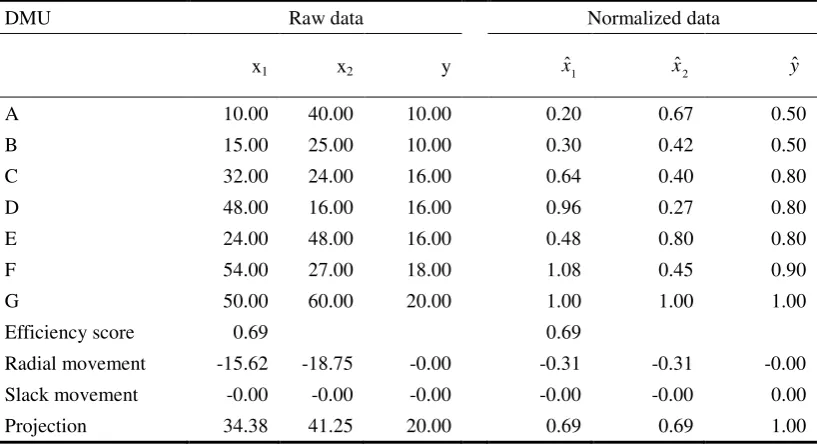
In order to prove empirically the consistency of the efficiency scores when normalized data are incorporated in units-invariant DEA models, we refer to Table 1. The testing sample consists of seven DMUs with two inputs (x1 and x2) and one output (y). Let DMU G be the unit under
evaluation (DMUo) and apply the input-oriented CRS model to original (raw) and normalized data.
The normalized data illustrated in Table 1 are calculated using formula (1). The efficiency score obtained from raw data is identical with the score that resulted from the utilization of normalized data. In a radial model, radial movement (-0.31) represents the degree of inefficiency.
Table 1. Illustration of DEA data normalization: efficiency measurement of DMU G using the
input-oriented CRS model
DMU Raw data Normalized data
x1 x2 y xˆ1 xˆ2 yˆ
A 10.00 40.00 10.00 0.20 0.67 0.50
B 15.00 25.00 10.00 0.30 0.42 0.50
C 32.00 24.00 16.00 0.64 0.40 0.80
D 48.00 16.00 16.00 0.96 0.27 0.80
E 24.00 48.00 16.00 0.48 0.80 0.80
F 54.00 27.00 18.00 1.08 0.45 0.90
G 50.00 60.00 20.00 1.00 1.00 1.00
Efficiency score 0.69 0.69
Radial movement -15.62 -18.75 -0.00 -0.31 -0.31 -0.00
Slack movement -0.00 -0.00 -0.00 -0.00 -0.00 0.00
Projection 34.38 41.25 20.00 0.69 0.69 1.00
3. Efficiency measurement using the directional distance function model
The linear programming of the directional distance function model is defined as follows
m ax
0
s.t. X v x
0
[image:7.595.98.507.369.591.2]7
, ,u 0 (14)
where v and u denote the input and output direction vectors, respectively.
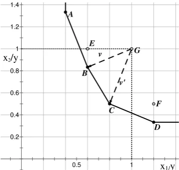
In directional distance function models, direction vectors determine the directions of movement of the inputs and outputs of the inefficient DMUs and target values (projections on the frontier), thereby determining efficiency scores. Direction vectors also reflect the relative importance of inputs and outputs in efficiency measurement. Figure 1 illustrates the impact of direction vectors on efficiency measurement drawing on an input-oriented CRS directional distance function model using normalized data.
0.5 1
1.4
1.2
1
0.8
0.6
0.4
0.2
v
v'
∙ ∙ ∙ ∙ ∙ ∙ ∙
∙ ∙ ∙ ∙ ∙ ∙ ∙
∙ ∙
∙ ∙
x2/y
x1/y
)
G
F E
D C
[image:8.595.211.389.258.427.2]B A
Figure 1. An input-oriented CRS directional distance function model using normalized data
In Figure 1, the horizontal coordinate represents the consumption of x1 for each unit of output and
the vertical coordinate represents the consumption of x2 for each unit of output. When the direction
vector is parallel to the horizontal axis, i.e., v = (1, 0), improvement is applied solely to x1, and the
efficiency score is determined exclusively by the inefficiency of x1. Similarly, when direction
vector is parallel to the vertical axis, i.e., v = (0, 1), improvement is associated only with x2, and the
efficiency score is determined exclusively by the inefficiency of x2. Furthermore, a downward
movement of the direction vector, i.e., from v to v’, indicates a decrease of the impact of x1 on the
measurement of the efficiency score and an increase of the impact of x2.
When the directional distance function models are incorporated in DEA, the inputs and outputs of DMUo usually are utilized as direction vectors. In such situations, directional distance function
models are equivalent to radial DEA models, and β, which reflects the degree of inefficiency, has the property of units-invariance. Unless the direction vectors are equal to the inputs and outputs of the DMU under evaluation, β is no longer units-invariant. Previous studies have not developed a solution for the problem of units-variance. As a result, the applicability of directional distance function models in efficiency measurement is limited.
8
1 1
1 1
1 1
1 1
1 1
1 1
m m
i i
m m
i i
q q
r r
q q
r r
v v
u u
m ax
0
ˆ ˆ
s.t. X v x
0
ˆ ˆ
Y u y
, ,u 0 (15)
where βv and βu represent the inefficiency of the inputs and outputs, respectively. The inefficiency score of the evaluated DMU is calculated as the arithmetical mean of the inefficiency scores of inputs and outputs.
In model (15), when the input direction vector v is set equal to the input vector of DMUo, i.e., v = (1,
1…, 1), and the output direction vector u is assigned a null vector, the model becomes equivalent to the input-oriented radial DEA model using normalized data, with efficiency score θ = 1-β. The efficiency score obtained from the application of model (15) is identical with the results obtained from radial models (4) and (8).
Alternatively, in model (15), by assigning a null vector to the input direction vector v, and setting the output direction vector u equal to the output vector of DMUo, i.e., u = (1, 1…, 1), the directional
distance function model becomes equivalent to the output-oriented DEA model using normalized data. In this case, the efficiency score is defined as θ = 1/(1+β). The efficiency score calculated by the directional distance function model (15) is identical with the results provided by radial models (5) and (9).
Theorem 1: For the data set illustrated in Table 1, if the length of the direction vector changes and the direction of the same vector is unchanged, then the efficiency remains unchanged.
Proof: Assume that the direction vectors of input and output are scaled up proportionally from v
and u to bv and bu, respectively, with b being a positive real number, and the Euclidian directions of the vectors are unchanged. Thus, model (15) becomes
1
1
1
1
1
1
m
i m
i q
r q
r
b v
b u
m ax b
0
ˆ ˆ
s.t. X b v x
0
ˆ ˆ
9
, ,u 0 (16)
If we let α be equal to βb
1 1 1 1 1 1 m i m i q r q r v u m ax 0 ˆ ˆ
s.t. X v x
0
ˆ ˆ
Y u y
, ,u 0 (17)
Model (17) is equivalent to model (15), so the efficiency scores they produce will be identical.
Theorem 2: For the same data set, model (15) is equivalent to model (18) shown below
1 1 1 1 m in 1 1 m i m i q r q r v u 0 ˆ ˆ
s.t. X v x
0
ˆ ˆ
Y u y
, ,u 0 (18)
Proof: Using normalized data, the inputs and outputs of the evaluated DMUs are all equal to unity. We know from the constraint condition of model (18) that
1
0 1 / m ax(v , ...,vi),i 1, 2, ...,m
Considering the interval of β, the numerator in model (18) is a monotonic decreasing function, while the denominator is a monotonic increasing function. As a result, within the interval of β, θ is regarded as a monotonic decreasing function. Therefore, model (18) is equivalent to model (15).
Acknowledging that model (18) is a nonlinear programming model, model (15) should be used instead for the measurement of efficiency when the directional distance function is incorporated. On the basis of model (15) we can introduce weights to inputs and outputs according to their relative significance in the efficiency measurement. To be more precise, model (19) is presented
10
m ax
0
ˆ ˆ
s.t. X v x
0
ˆ ˆ
Y u y
, ,u 0
1 1 , q m i r i r
w m w q (19)
where w stands for the weight assigned to inputs, and h indicates the weight of outputs.
Efficiency measurement can be extended to cases with undesirable outputs. Namely, when undesirable outputs are present, the directional distance function model is defined as follows
1
1
' ' 1
1 ' 1
' ' 1 ' ' ' 1 1 i m i i m q q r r q r r r r q w v
h u h u
' ' ' m ax s.t. k k k
X v x
Y u y
Y u y
' '
1 1 1
, ,
q q
m
i r t
i r t
w m w q w q
' 1 (20)
where q' denotes the number of undesirable outputs incorporated in the model, h' stands for the weight of undesirable outputs, u' expresses the direction vector of undesirable outputs, and ω and ω’ are the weights that determine the mix of desirable and undesirable outputs, respectively, in the measurement of efficiency.
4. Concluding remarks
11
References
Banker, R. D., Charnes, A., & Cooper, W. W. (1984). Some models for estimating technical and scale
inefficiencies in data envelopment analysis. Management Science, 30, 1078-1092.
Chambers, R. G., Chung, Y., & Färe, R. (1996). Benefit and Distance Functions. Journal of Economic
Theory, 70, 407-419.
Chambers, R. G., Chung, Y., & Färe, R. (1998). Profit, directional distance functions, and Nerlovian
efficiency. Journal of Optimization Theory and Applications, 98, 351-364.
Charnes, A. (1994). Data envelopment analysis: theory, methodology, and application: Kluwer
Academic Publishers.
Charnes, A., Cooper, W. W., & Rhodes, E. (1978). Measuring the efficiency of decision making units.
European Journal of Operational Research, 2, 429-444.
Chung, Y. H., Färe, R., & Grosskopf, S. (1997). Productivity and undesirable outputs: A directional
distance function approach. Journal of Environmental Management, 51, 229-240.
Cook, W. D., & Seiford, L. M. (2009). Data envelopment analysis (DEA) - Thirty years on. European
Journal of Operational Research, 192, 1-17.
Färe, R., & Knox Lovell, C. A. (1978). Measuring the technical efficiency of production. Journal of
Economic Theory, 19, 150-162.
Lovell, C. A. K., & Pastor, J. T. (1995). Units invariant and translation invariant DEA models.
Operations Research Letters, 18, 147-151.
Seiford, L. M. (1996). Data envelopment analysis: The evolution of the state of the art (1978–1995) The
Journal of Productivity Analysis, 6, 99-137.
Tone, K. (2001). A slacks-based measure of efficiency in data envelopment analysis. European Journal
![A Molecular Electron Density Theory Study of the Reactivity of Azomethine Imine in [3+2] Cycloaddition Reactions](data:image/gif;base64,R0lGODlhAQABAIAAAP///wAAACH5BAEAAAAALAAAAAABAAEAAAICRAEAOw==)