Euler Maclaurin Expansions of Errors for Multidimensional Weakly Singular Integrals and Their Splitting Extrapolation Algorithm*

http://www.scirp.org/journal/jamp ISSN Online: 2327-4379

ISSN Print: 2327-4352

DOI: 10.4236/jamp.2017.52022 February 15, 2017

Euler-Maclaurin Expansions of Errors for

Multidimensional Weakly Singular Integrals

and Their Splitting Extrapolation Algorithm

*

Yubin Pan, Jin Huang, Hongyan Liu

School of Mathematical Sciences, University of Electronic Science and Technology of China, Chengdu, China

Abstract

In this paper, multidimensional weakly singular integrals are solved by using rectangular quadrature rules which base on quadrature rules of one dimen-sional weakly singular and multidimendimen-sional regular integrals with their Eu-ler-Maclaurin asymptotic expansions of the errors. The presented method is suit for solving multidimensional and singular integrals by comparing with Gauss quadrature rule. The error asymptotic expansions show that the con-vergence order of the initial quadrature rules is

( )

i 1

i

O hα+ , where − ≤1 αi ≤0.

The order of accuracy can reach to

( )

4 0

O h by using extrapolation and split-ting extrapolation, where h0 is the maximum mesh width. Some numerical

examples are constructed to show the efficiency of the method.

Keywords

Multidimensional Weakly Singular Integrals, Euler-Maclaurin Errors Asymptotic Expansions, Splitting Extrapolation

1. Introduction

It is well known that multidimensional singular integrals are models arising in diverse engineering problems and mathematical applications. For example, in the boundary element fracture analysis problem, elasticity problem [1], bima-terial interfacial cracks [2] and wedge-sharped bimabima-terial interface [3], etc. Few of these integrals and equations can be solved explicitly, it is necessary to find a good numerical method. At present, there are many numerical techniques to calculate one-dimensional singular integrals or integral equations, such as collo-cation method [4], Gaussian quadrature method [5] [6], mechanical quadrature

*This work was supported by the National Natural Science Foundation of China (11371079). How to cite this paper: Pan, Y.B., Huang,

J. and Liu, H.Y. (2017) Euler-Maclaurin Expansions of Errors for Multidimensional Weakly Singular Integrals and Their Split-ting Extrapolation Algorithm. Journal of Applied Mathematics and Physics, 5, 252- 258.

https://doi.org/10.4236/jamp.2017.52022 Received: December 3, 2016

method [7] [8]. The Gauss-quadrature rules are considered to be a good choice for solving high dimensional integrals because they were accurate for polynomial approximation and the cost is low. However, Gaussian formula is not suitable for dealing with more than five-dimensional problems. So, we give a new algo-rithm for solving the following integral

( )

(

)

1

(

)

1 1

1

, , d d ,

s s

b b

s s

a a

I F x =

∫ ∫

 F x  x x x (1)

where

(

)

(

1

)

[

]

1

1

, ,

, , _s s ,_{i i}, _i , 0 _i 1, 1, ,

s i i i i

f x x

F x x t a b i s

x t α

α

=

= ∈ < < =

Π −



  .

The structure of this paper is as follows: In Section 2, we give quadrature rules for weakly singular integral with multivariate errors asymptotic expansions. In Section 3, we construct the splitting extrapolation algorithm. In Section 4, some examples are given to illustrate the validity of the proposed method. Section 5 concludes the paper with a brief summary.

2. Multi-Parameters Asymptotic Expansions of the Errors

for Weakly Singular Integrals

In this part, we mainly consider multidimensional weakly singular integrals. We give the corresponding results of multidimensional weakly singular integrals ac-cording to the quadrature formula and asymptotic expansions of the errors of one-dimensional integrals.

Theorem 1. If

(

)

2

1, ,

l s

f x  x ∈C on the interval

[

a b₁, ₁

]

× ×

[

a bs, s

]

, and

we assume that

(

)

(

1

)

[

]

1

1

, ,

, , , , , 1, ,

i

s

s _s i i i i i i

f x x

F x x t a b i s

x t α

=

= ∈ =

Π −



  ,

(

)

(

1

)

1 1

1 1

, ,

, ,

i

s s

f x x

F x x

x t α

= −



 ,

(

)

(

1

)

2 1

2

, ,

, ,

i

s s _s

i i i

f x x

F x x

x t α

= =

Π −



 ,

( )

(

)

1

(

)

1 1

1

, , dx d

b _bs

s s

a _as

I F x =

∫ ∫

 F x  x  x, 0< <αi 1. Then we have the following asymptotic expansions of the errors

( )

(

( )

)

( )

2 2 1

( )

2

0

1 | | 1 0 | | 1

,

l

l l

E I F Q A B + + O h

≤ ≤ − ≤ ≤ −

= − =

∑

μ+

∑

μ α +

μ μ

h x h h h (2)

where h=

(

h1,,hs

)

, h0=max1≤ ≤i s

{

h1,,hs

}

,

i i i

i

b a

h N

−

= , i=1,,s,

(

)

{

1 0, , , , 0 , 0 or 1

}

s

i i i i i

i=k e e

α

k

=

∑

=   =

α .

Proof: We prove the theorem by the mathematic induction method. First, the conclusion is obvious right for k=1. Now, we assume that the result also holds

when k= −s 1. Next, we just need to prove the case of k=s

(

)

(

)

(

)

( )

( )

( )

1 2

1 2

1

1 2

1

1 1 1

1

1 1

1 1 1 2

1 2 2

2 1

1 1 2 2

2 2 1 2

1 1 0

1 | | 1 0 | | 1

, , 1 , ,

d d

, , ,

1 1

,

s s

i s

s

b b_{s s} b b b _s

s

s _s

a as a a a i

i i i i i i

N N

b _{i si}

s a

i i _{s s}

l

l l

f x x f x x

x x

x t x t x t

f x x x

h h

x t x t x t

A x B x O h

α α

α α α

= =

= =

+ +

≤ ≤ − ≤ ≤ −

=

Π − − Π −



= 

− _ − −



+ + + _



∫

∫

∫

∫

∫

∑

∑

∫

∑

∑

 

  

 

μ μ α

μ μ

μ μ

h h

where h=

(

h2,,hs

)

, Aμ

( )

x1 , Bμ

( )

x1 are functions which are independent

of h. The integral can be written as

( )

(

)

(

)

( )

( )

2 1

2 ₁ 1

1 1 ₁

1 1 1 1 1 1 1 1 2 2 1

1 _{2 2} 1 _{1 1}

( ) 1

2 2 1

1 1

1 | | 1 _{1 1} 0 | | 1 _{1 1}

2

0 1

1 1

1 2 3 4

, , , 1 1 d d d 1 d , s s N N

b _{i si}

s _a

i i _{s s}

b b x

a a

l l

b l

a

f x x x

I F h h x

x t x t x t

B

A x

x x

x t x t

O h x

x t

I I I I

α α α

α α α = = + + ≤ ≤ − ≤ ≤ − = − − − + + − − + − = + + +

∑

∑

∫

∑

∫

∑

∫

∫

  μ μ

μ μ α

μ μ

x

h h

(4)

we consider I1

(

)

(

)

( )

2 1 2 ₁ 2 1 2 1 2

1 2 ₁ 1

2 _{2 2} 1 _{1 1}

1

2 1 ₁

1 _{2 2} 1 1 _{1 1}

1 1

2 1

2 ₁ 2

1 1 1

1 1

11 12 13 14

, , , 1 1 d , , 1 1 , s s s s N N

b _{i si}

s _a

i i _{s s}

N

N N

i si s

i i _{s s} i

l l

l

f x x x

I h h x

x t x t x t

f x x

h h h

x t x t x t

Ah Bh O h

I I I I

α α α

α α α

µ α µ µ µ = = = = = − − + + = = = − − −  =  − − _ −  + + + _  = + + +

∑

∑

∫

∑

∑

∑

∑

∑

    (5)

then I11 can be represented as

(

)

1

1 11 1

1

1 _{1 1} 1

, , 1 . s N N i si s

i i i si s

f x x

I h h

x t

x t α

= =

=

− −

∑



∑

 (6)

We need to consider the following formula

( )

2 2 2 2 2

2 _{2 2} 1

2 2 1 2

2 0

1 | | 1 0 | | 1

2

1 1

1

d d ,

s s s i s N N s

i i _{s s}

b b _l

s s

a a

l l

i i i

h h

x t x t

x x A B O h

x t α α α = = + + ≤ ≤ − ≤ ≤ − = − − = + + + Π −

∑

∑

∑

∑

∫

∫



  μ μ α

μ μ

h h

(7)

we know the above equation is obviously right by induction. Next, we calculate

12 I

( )

( )

2 2 2 2 1 2

12 2 1

2 _{2 2} 1 1

1 2

1 2

1 ₂

2 2 1 2

0 1 | | 1 0 | | 1

1

2 2 2 1 2

1 1 2 1 0

1 1 | | 1 0 | | 1

1 1 1 d d . s s s i s N N l s

i i _{s s} l

b b

s s

a a

i i i

l

l l

l

l

l l

I h h Ah

x t x t

Ah x x

x t

A B O h

A h A B O h

µ α α µ µ α µ µ µ − = = = − = ₌ + + ≤ ≤ − ≤ ≤ − − + + = ≤ ≤ − ≤ ≤ − = − −  = _ Π −   + + + _  = + + +

∑

∑

∑

∑

∫

∫

∑

∑

∑

∑

∑

  

μ μ α

μ μ

μ μ α

μ μ

h h

h h

(8)

The same as I12 we can easy obtain

( )

1

2 ₁1 2 2 1 2

13 2 1 3 3 0

1 1 | | 1 0 | | 1

,

l

l

l l

I B h µ α A B O h

µ

− _{+ +}

+ +

= ≤ ≤ − ≤ ≤ −

=

∑

+

∑

μ+

∑

μ α +

μ μ

( )

2

14 0 .

l

I =O h (10)

Now, we consider I I I2, 3, 4

( )

1 1 1 1 2 2

2 1 4

1 | | 1 _{1 1} 1 | | 1

d ,

b a

l l

A x

I x A

x t α

≤ ≤ − ≤ ≤ −

= =

−

∑

μ

∫

μ

∑

μ

μ μ

h h (11)

( ) 1

2 1 1 2 1

3 1 4

1 1

0 | | 1 _{1 1} 0 | | 1

d , b x alpha a l l B

I x B

x t

+ + + +

≤ ≤ − ≤ ≤ −

= =

−

∑

_{μ α}

∫

μ

∑

_{μ α}

μ μ

h h (12)

( ) ( )

1

1 1

2 2

4 1 0 0

1 1

1

d .

b _{l l}

a

I x O h O h

x t α

= =

−

∫

(13)

Now, we obtain the following equation by taking the I I I I1, 2, 3, 4 and I11,I12,

13, 14

I I into Equation (4)

( )

(

)

(

( )

( )

)

2 2 1

( )

2

0

1 | | 1 0 | | 1

,

l

l l

I F Q F x A B + + O h

≤ ≤ − ≤ ≤ −

− =

∑

μ+

∑

μ α +

μ μ

x h h (14)

where A B, are constant which are independent of h=

(

h₁,,h_s

)

. The proof has been completed. 

3. Splitting Extrapolation Algorithm

Now, we introduce the splitting extrapolation algorithm

( )

( )

( )

(

)

(

)

1 2 2

1 1 2 | | 2

2 1 2 1

0 0 | | 2

ln ,

s s

i

h i i i i

i i m

m m

I f Q f A h B h A

B O h α + = = ≤ ≤ ′ + + + ≤ ≤ = + + + + +

∑

∑

∑

∑

μ μ μ δ μ α μ μ h h h (15)

where

( )

1

(

(

)

(

)

)

1

1 1

1 0 0 1 1 1, ,

s s

n n

h s i i s s s

Q f =hh

∑

₌−

∑

₌− f i +

β

h  i +

β

h ,

(

)

{

1 0 or 1, 0, , , , 0 , 1 2

}

s

i i i i i s

i=k e k e

α

k k k

′ =

∑

= =   = + + ≥

α .

First, we have to eliminate the minimum term of the errors expansions. Ac-cording to (2), we can easily find that i 1

i

hα+ , i=1,,s are low order terms

when μ =0. Assuming that αi+ =1 min1≤ ≤j s

{

αj+1

}

, and we use splitting extra-

polation in the direction of xi

( )

(

)

1 (0) 2 1,1 1 1, 1, 1 2 2 2 1 1 2 | | 2

2 1

2 1

21 1 1 1 2 1

1 0

0 | | 2

, , , , 2

2 2 2

,

2

s s

j i

s j j j j

j j i j j i

i i

i i i s

i i s

m k i i i

k

k i s s s m

s m

h

I f Q h h A h B h

h h h

A B A h h

h

B h h O h

α α µ µ µ µ α µ α µ α + = ≠ = ≠ + ≤ ≤ + + + + + + + ≤ ≤   = _{ }+ +         + _{ }+ _{ } + _{ }         + _{ } +  

∑

∑

∑

∑

      μ μ μ μ (16)

Then, we use

(

1 (0)

( ) ( )

) (

1

)

1,1

2αi+ _{I f} −_{I f} 2αi+ −1 and obtain the following equa-tion

( )

(

)

(

)

(

)

1

(1) (1) 2

1,1 1,1 1 ,1 ,1

1, 1,

1 2 1

2 2 1

,1 ,1 0

0 | |< 2

, ,

lni ,

s s

j

s j j j j

j j i j j i

m i

i i i i i

m

I f Q h h A h B h

where

(

)

1

1 1

(1)

1,1 1

2 , , , , , ,

2

2 1

i i

s s

i

h

Q h h Q h h Q

α

α +

+

 _{ −}

 

 

=

−

  

, and Ai,1,Bi,1,i=1,,s are

constants which are unrelated to h. We can obtain higher accuracy and

con-vergence order by repeating the above process.

4. Examples

In this section, we give some examples to illustrate the efficiency of the proposed method.

Example 1. We consider the following s-dimensional integral [9]

(

)

(

)

1 1

1 1

0 0exp d d 1 .

s

s s

x + +x x x = −e

∫ ∫

   (18)

We give the numerical results of the splitting extrapolation of types 1 and 2 and Gauss quadrature methods. Table 1 gives the relative error (RE) and CPU time for different dimension (s) and splitting times (m). From the Table 1, we

can find that the splitting extrapolation method is suit for solving high dimen-sional integrals, and Gauss quadrature rule is difficult for solving more than five dimensional problems.

Example 2. we consider the following integral

(

) (

) (

)

(

(

( )

)

)

1/3

1/3 1/3 1/2

1 2 3 4

1 1 1 2 2 2 3 8/15 2/3

1 7

1/4 1/4 1/5

0 0 0 1 1 1 1

5 6 7

3 2

d d 6 2 1 1 .

1 1 1

x x x x

x x

x x x

−

− − −  ₋ 

 

  _{= − − −}

− − −

∫ ∫ ∫ ∫ ∫ ∫ ∫

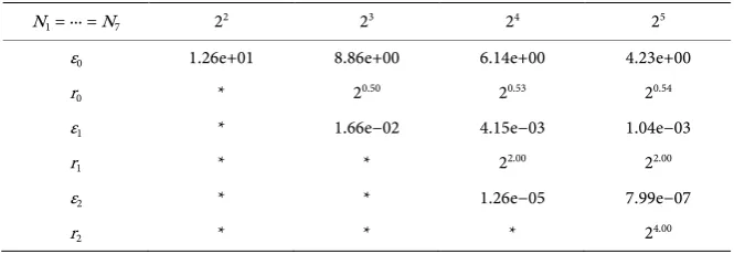
 (19)

This is a high dimensional weakly singular integral which can be solved by splitting extrapolation algorithm. In Table 2, we give the absolute errors and convergence orders for splitting extrapolation of each step. From the table, we can find that the convergence order can reach to

( )

4

0

[image:5.595.207.540.623.738.2]

O h by using splitting extrapolation twice, and the orders are coincide with the theoretical analysis. In Figure 1, we give the curves of absolute errors for each splitting extrapolation. From the Vertical direction, the images sink and the slopes of the curves increase with the increasing of the splitting times, which indicates that the errors decrease and the convergence orders increase. From the horizontal coordinate, the errors are reduced with the increasing of the node numbers. This shows that the split-ting extrapolation not only enhance the numerical precision but also the order of accuracy.

Table 1. Numerical results with errors and orders of accuracy for Example 2.

N1 = ∙∙∙ = N7 22 23 24 25

ε0 1.26e+01 8.86e+00 6.14e+00 4.23e+00

r0 * 20.50 20.53 20.54

ε1 * 1.66e−02 4.15e−03 1.04e−03

r1 * * 22.00 22.00

ε2 * * 1.26e−05 7.99e−07

[image:6.595.208.540.86.421.2]

Table 2. The compare between SE and Gauss quadrature method.

s m Type 1 Type 2 Gauss RE CPU(s) RE CPU(s) RE CPU(s) 5 7 8.6e−13 335 5.0e−9 336 1.0e−8 42

8 1.9e−13 947 1.2e−8 656 1.0e−9 >9 h 8 5 3.7e−7 618 3.7e−7 502 4.1e−8 11,283

6 9.7e−9 4056 9.4e−9 3092

9 4 2.1e−5 176 2.1e−5 144 1.0e−3 >8 h 5 8.5e−7 1544 8.6e−7 1197

Figure 1. The absolute errors of splitting extrapolation.

5. Conclusion

In this paper, we give the quadrature formula with the asymptotic expansions of errors for solving multidimensional integrals with arbitrary points weakly sin-gular. According to the asymptotic expansions of errors, we construct splitting extrapolation algorithm to improve the accuracy and the convergence order of the numerical results. By comparing the numerical results of our method with Gauss quadrature method, we can conclude that the splitting extrapolation me-thod is efficient for solving high dimensional integral and weakly singular inte-grals. Next, we consider how to use the method to deal with boundary integral and differential equations.

Acknowledgements

The authors are very grateful to the referees and editors. This work was partially supported by the financial support from National Natural Science Foundation of China (Grant no. 11371079).

References

Mathematical, Physical and Engineering Sciences, No. 458, 2721-2733.

[2] Rice, J. (1988) Elastic Fracture Mechanics Concepts for Interfacial Cracks. Journal of Applied Mechanics, 55, 98-103. https://doi.org/10.1115/1.3173668

[3] Bogy, D. (1971) Two Edge-Bonded Elastic Wedges of Different Materials and Wedge Angles under Surface Tractions. Journal of Applied Mechanics, 38, 377-386.

https://doi.org/10.1115/1.3408786

[4] Chrysakis, A.C. and Tsamasphyros, G. (1992) Numerical Solution of Integral Equa-tions with a Logarithmic Kernel by the Method of Arbitrary Collocation Points. In-ternational Journal for Numerical Methods in Engineering, 33, 143-148.

https://doi.org/10.1002/nme.1620330110

[5] Milovanovic, G.V. and Spalevic, M.M. (2006) Quadrature Rules with Multiple Nodes for Evaluating Integrals with Strong Singularities. Journal of Computational and Ap-plied Mathematics, 189, 689-702. https://doi.org/10.1016/j.cam.2005.05.021

[6] Rathod, H.T., Venkatesudu, B., Nagaraja, K.V., et al. (2007) Gauss Legendre-Gauss Jacobi Quadrature Rules over a Tetrahedral Region. Applied Mathematics and Com-putation, 190, 186-194. https://doi.org/10.1016/j.amc.2007.01.014

[7] Jin, H. and Tao, L. (2004) The Mechanical Quadrature Method and Their Extrapola-tion for Solving BIE of Steklov Eigevalue Problem. Journal of Computational Ma-thematics, 22, No. 5.

[8] Lyness, J.N. (1976) Applications of Extrapolation Techniques to Multidimensional Quadrature of Some Integrand Functions with a Singularity. Journal of Computa-tional Physics, 20, 346-364. https://doi.org/10.1016/0021-9991(76)90087-5

[9] Lv, T. (2015) A High Accuracy Extrapolation Algorithm for Multi-Dimensional Problems. China Science Publish.

Submit or recommend next manuscript to SCIRP and we will provide best service for you:

Accepting pre-submission inquiries through Email, Facebook, LinkedIn, Twitter, etc. A wide selection of journals (inclusive of 9 subjects, more than 200 journals)

Providing 24-hour high-quality service User-friendly online submission system Fair and swift peer-review system

Efficient typesetting and proofreading procedure

Display of the result of downloads and visits, as well as the number of cited articles Maximum dissemination of your research work

Submit your manuscript at: http://papersubmission.scirp.org/