A Wavelet Multigrid Method Using Symmetric
Biorthogonal Wavelets
Doreen De Leon
Department of Mathematics, California State University, Fresno, USA Email: [email protected]
Received March 24,2013; revised April 25, 2013; accepted May 23, 2013
Copyright © 2013 Doreen De Leon. This is an open access article distributed under the Creative Commons Attribution License, which permits unrestricted use, distribution, and reproduction in any medium, provided the original work is properly cited.
ABSTRACT
In [1], the author introduced a wavelet multigrid method that used the wavelet transform to define the coarse grid, in-terpolation, and restriction operators for the multigrid method. In this paper, we modify the method by using symmetric biorthogonal wavelet transforms to define the requisite operators. Numerical examples are presented to demonstrate the effectiveness of the modified wavelet multigrid method for diffusion problems with highly oscillatory coefficients, as well as for advection-diffusion equations in which the advection is moderately dominant.
Keywords: Multigrid; Wavelets; Biorthogonal Wavelets
1. Introduction
It is well known that the multigrid method is very useful in increasing the efficiency of iterative methods used to solve systems of algebraic equations approximating par-tial differenpar-tial equations. However, when confronted by certain problems, for example diffusion problems with discontinuous or highly oscillatory coefficients, the stan-dard multigrid procedure converges slowly, with a rate dependent on the initial mesh size, or may even break down.
In [2], the wavelet transform, which uses both high- and low-pass filter operators, is used to derive a new ap-proach for the two-level multigrid method, under the assumption that the matrix on the fine grid is symmetric. Some one-dimensional examples are also examined in that paper. In [1,3], the author extended the results of this approach to two dimensions and to multiple-level multi-grid, dropping the assumption of a symmetric fine grid operator. This approach was considered for several rea-sons. First, in [4], the authors investigate similarities be-tween multiresolution analyses and multigrid methods, which similarities motivate investigation into wavelet- based multigrid methods. In addition, in [5], for example, it is shown that a wavelet coarse grid operator defined by a Schur complement provides a good approximation to the homogenized coarse grid operator, and, as stated in [1,3], homogenization has been used to improve conver-gence of multigrid methods for diffusion problems with
periodic coefficients (e.g., [6-9]) because the homoge- nized operator provides a very good approximation of the important properties (e.g., eigenvalues and eigenfunc- tions) of the original fine grid operator. Also a wavelet coarse grid operator defined by a Schur complement has a natural connection to the interpolation and restriction operators. Furthermore, wavelets can be applied to prob- lems with periodic as well as non-periodic coefficients. Finally, the application of wavelet operators to vectors and matrices maintains the properties of the original problem.
method which they use to solve various partial differen-tial equations.
In this paper, the wavelet multigrid method introduced in [1] is modified by using symmetric biorthogonal wavelet transforms to define the requisite operators. The organization of this paper is as follows. In Section 2, some background on multigrid methods and wavelets is given. Section 3 discusses the wavelet multigrid method developed from the application of the biorthogonal wavelet transform to a general second order partial dif-ferential equation in two dimensions. In Section 4, nu-merical considerations are discussed. Section 5 presents some numerical results of applying the modified wavelet multigrid method using symmetric biorthogonal wavelets to two diffusion problems with highly oscillatory coeffi-cients and to three advection-diffusion problems with moderately dominant advection. The rapid convergence, relatively independent of the initial mesh size, of the modified wavelet multigrid method using biorthogonal wavelets is demonstrated for these problems. For all nu-merical results in this paper, the V-cycle multigrid method is used with one iteration of the smoother for the coarsening and the correcting phases.
2. Background
2.1. Multigrid Methods
The problem we are concerned with solving is the system of linear equations
,
Aub (1)
where A and arise from discretization of a (partial)
differential equation on some grid , where is the step size.
b
h
h
We briefly describe the V-cycle method used in this paper. Given some interpolation operator, 2 ,
h h
I where
the superscript refers to the fine grid and the subscript refers to the coarse grid, and a restriction operator, 2h,
h
I
we can define a multigrid method recursively. For the two-level V-cycle method, we do the following.
Step 1: Relax a few (usually one or two) steps on the fine grid h to get an initial guess h.
u
Step 2: Compute the residual and restrict the residual to the coarse grid .
h h h
r b A u
2h, 2h 2h h
r I
2he2h 2h h
h
r
Step 3: Solve the error equation A r on the
coarse grid.
Step 4: Set and again relax a few (usually one or two) steps on the fine grid.
2 2 e
h h h h
u u I h
Based on this two-level method, the V-cycle multigrid scheme is defined recursively. Some good references for multigrid methods are [17-19].
One type of multigrid scheme is algebraic multigrid, which only uses the structure of the matrix in the prob-lem to determine the coarsening process (choice of coarse
grid and definition of interpolation/restriction operators). This process is performed in order to ensure that the range of interpolation approximates the errors not suffi-ciently reduced via relaxation. For a more detailed de-scription of algebraic multigrid methods, see, e.g., [19- 22]. Note that in [21] the relationship between algebraic multigrid and Schur complements is discussed. Algebraic multigrid methods are of particular interest, in that they are the nearest methods to the approach used for the wavelet multigrid method.
It is expected that the multigrid method should con-verge at a rate independent of the fine mesh size. How-ever, for certain problems, including elliptic problems with highly oscillatory coefficients, such convergence does not occur for the standard multigrid method. One difficulty is that the small eigenvalues of A are not
nec-essarily associated with smooth eigenfunctions, a key assumption for the standard multigrid method. For such problems, it is not as simple to approximate the smooth eigenfunctions on the coarse grids. New methods for restriction and interpolation, or for treating the entire problem, must be found. One such approach is the wave-let multigrid method discussed in [1,3] and the modified wavelet multigrid method discussed in this paper.
2.2. Wavelets and Biorthogonal Wavelets
For background, a brief description of wavelets, and then of biorthogonal wavelets, follows. For more details, the reader is referred to [10,23-25].
2.2.1. Wavelets
Wavelets basically separate data (or functions or opera-tors) into different frequency components and analyze them by scaling. The wavelets can be chosen to form a complete orthonormal basis of 2
L . Due to the
scal-ing of the wavelet functions, they have time- or space- widths that are related to their frequency: at high fre-quencies, they are narrow, and at low frefre-quencies, they are broader. Therefore, they provide good localization of functions in both the frequency domain and physical space, and representation by wavelets seems natural to apply to the analysis of fine and coarse scales.
A multiresolution analysis (MRA) consists of a se- quence of closed subspaces VjVj1 of
2
L , the
scaling spaces, that satisfy certain conditions. For every
,
j Wj is defined as the orthogonal complement of
j
V in Vj1. The Wj are called the wavelet spaces.
Define Hj and Gj to be the operators that transform
the basis of the space Vj to the bases of the spaces Vj1
and Wj1, respectively. The properties of Hj and Gj
(assuming Hj and Gj are real-valued) are
(i) T T
j j j j
H H G G I.
(ii) T T 0
j j j j
(iii) T T
j j j j
H H G G I.
j
H and Gj can be thought of in terms of filter
theory, with Hj being a low-pass filter (i.e., allowing
only low frequency values to pass) and Gj being a
high-pass filter (i.e., allowing only high frequency values
to pass). The wavelet transform, j:VjVj1Wj1,
is defined by
. j j
j H
G
Note that j is orthogonal due to the properties of j
H and Gj.
In the discrete context, the wavelet operators are computationally efficient. With respect to the Haar mul-tiresolution analysis, application of the low-frequency operator
Hj to a vector in involves onlyoperations. The same holds for the high-frequency op-erator
n
2n
Gj 4. So, the application of the wavelet transform requires only operations. In general, application of the wavelet transform requires operations, as-suming a finite number of coefficients for the low- and high-frequency operators.
n
n
In two dimensions, the tensor product of one-dimen- sional multiresolution analyses is used. So Vj is
de-fined by VjVjVj. These spaces Vj then form an
MRA in 2
2 . For each ,L j Wj is defined as the orthogonal complement of Vj in Vj1. So,
1 1 1
.
j j j
j j j j j j j j
j j
V V
V V W V V W W W
V
V W
(2)Then, analogous to the one dimensional case, define the operators Hj and Gj so that
y x
j j j
H H H
and
.
y x j j y x
j j j
y x j j
G H
G H G
G G
j
H and Gj have the same properties as their one-
dimensional analogues. As in the one-dimensional case, the wavelet transform, j:VjVj1Wj1, is defined
by
.
j j
j
H G
Again, due to the properties of Hj and Gj, j is
orthogonal.
2.2.2. Biorthogonal Wavelets
A biorthogonal multiresolution analysis consists of two
dual multiresolution analyses. In other words, there are two dual sequences of closed subspaces of 2
L ,
1and 1,
j j j j
V V V V
both of which satisfy the conditions of a multiresolution analysis. For every j, Vj1 can be written as the direct sum of Vj and Wj, and Vj1 can be written as
the direct sum of Vj and Wj. Wj and Wj are
de-fined so that their biorthogonal basis functions, the wavelets
j x
and j
x , respectively, satisfycer-tain conditions including forming a Riesz basis of
2
L . For symmetric biorthogonal multiresolution
analyses, these wavelet bases (and the bases for the scal-ing spaces) are symmetric. Define Hj and Gj to be
the operators that transform the basis of the space Vj to
the bases of the spaces Vj1 and Wj1, respectively;
and define Hj and Gj to be the operators that
trans-form the basis of the sp e ac Vj to the bases of the spaces 1
j
V and Wj1, respectively. The propertie ofs Hj, j
G , Hj and Gj are as follows:
(i) T T
j j j j
H H G G I.
(ii) T T 0
j j j j
H G G H .
(iii) T T
j j j j
H H G G I.
The wavelet transform, j:VjVj1Wj1
1 1
and the dual transform j: j j Wj
V V
H
are defined by
and ,
j j
j j
j j
H
G G
where we use to denote the direct sum for ease of notation. Note that j is orthogonal to j due to the properties of Hj, Gj, Hj and Gj. Also, note that in
terms of filter theory, Hj and Hj are low-pass filters,
and Gj and Gj are high-pass filters.
The discrete biorthogonal wavelet transforms are also computationally efficient, and application of these op-erators requires
n operations, assuming a finitenumber of coefficients for the low- and high-frequency operators.
In two dimensions, we use the tensor product in a similar way as for the standard multiresolution analysis. So, Vj is defined by VjVjVj and Vj is defined
by
j j
V V . These spaces Vj and Vj then form dual
MRAs in
2 2
L . Wj and Wj are defined so that
their basis functions are the tensor products of the one-dimensional wavelets and scaling functions. For each
j, Vj1 can be written as the direct sum of
j
V and Wj, and Vj1 can be written as the direct sum of Vj and Wj. So, we have
1 1 1
,
j j j
j j j j j j j j
j j
V V
V V W V V W W W
V
V W
fine grid, apply the wavelet transform j to both sides
of the equation and use the orthogonality of j with j
to obtain and similarly for Vj1, where we again use to
de-note the direct sum for ease of notation.
Then, analogous to the one-dimensional case, define
the operators Hj, Gj, Hj and Gj so that:
T
T ,
j j j j j
L L
LH LH
j j j
HL HL
HH HH
L u f
u f u f L u f u f
(5)
and ,
y x y x
j j j j j j
H H H H H H
and
and .
y x y x
j j j j
y x y x
j j j j j j
y x y x
j j j j
G H G H
G H G G H G
G G G G
where uL,fLVj and
, , and
j j j j
H G H G
1
:
have the same properties as their one-dimensional analogues. As in the one-dimensional case, the wavelet transform and the dual transform
T
T, , , , , .
LH HL HH LH HL HH j
u u u f f f W
The main idea for the remainder of the method follows in a similar manner as the wavelet multigrid method using orthogonal wavelet transforms. First, T
jLj j
ˆ is computed, and the resulting matrix, denoted by Lj, is
partitioned to obtain
1
j VjVj Wj 1
and j:VjVj1Wj , are
defined by and . j j j j j j H H G G T T T T T ˆ .
j j j j j j
j j j j
j j j j j j
j j
j j
H L H H L G
L L
G L H G L G
T B C D (6) Again, due to the properties of Hj, Gj, Hj and
j
G , j is orthogonal to j.
3. The Modified Wavelet Multigrid Method
Using Biorthogonal Wavelets
Then, the block UDL decomposition of ˆLj
1
ˆ
, where U
is block upper triangular with unit diagonal, D is block
diagonal, and L is block lower triangular with unit
diagonal, is computed and is used to find Lj
as follows. The block UDL decomposition of ˆLj is determined to
be The two-dimensional wavelet multigrid method was in-troduced in [3] and [1]. Both of these works assumed orthogonal wavelet operators. Here, we describe the modified wavelet multigrid method using biorthogonal wavelet transforms. For the work in this paper, the bior-thogonal wavelet transform is formed using symmetric
biorthogonal wavelets. 1
1 1 0 0 . 0 0
j j j j j j
j
j j j
I T B D C
I B D L
D C I D I
(7)
Given the problem
,
j
L u f (4)
The inverse of this factorization of ˆLj is then
computed, which after multiplication of the factors gives where Lj represents the operator obtained by
discretiz-ing a two-dimensional partial differential equation on the
1 1 1 1 1 1 11 1 1 1 1
ˆ j j j j j j j j j j ,
j
j j j j j j j j j j j j j j j
T B D C T B D C B D
L
D C T B D C D C T B D C B D D
1 1
where we observe that 1
j j j j
T B D C is the Schur complement of Dj in ˆLj. Define
. L L LH j H HL HH u u u v u u u u
Solving for gives v
1
1 1
1
1 1 1 1 .
j j j j j j j j
j j j j j j j j j j j j
T B D C H B D G
v f
D C T B D C H B D G D G
Since , T
T T
j j j j
v u u v H G v
. So,
T T 1 T
1
1 11
0
. 0
j j j j j j j j
j j j j j
j j
H B D G
T B D C
u H G D C G f
G D
(8)
Motivated by the work in [1], we denote
T T 12 2
h
h j j j j
I H G D C (9)
and
2 2
2
h
h j j j
1
j
I H B D G (10)
as the interpolation and restriction operators, respectively. Plugging the interpolation and restriction operators de-fined in (9) and (10) into (8) gives,
1
1 2 T 12 .
h h
h j j j j h j j j
uI T B D C I f G D G f (11)
In multigrid, the error correction on the coarse grid is sought, i.e., the equation being solved is (11) with u
re-placed by the error, e, and f replaced by the residual, r:
1
1 2 T 12 .
h h
h j j j j h j j j
eI T B D C I rG D G r
Assuming that T 1
j j j
G D G r is small, i.e., r is almost in
the error can be approximated by
TRange Hj ,
1
1 22 ,
h h
h j j j j h
eI T B D C I r
resulting in
1
22 .
h
j j j j h h h
T B D C e I r
The above assumption is good for most of the classical iterative methods, like Jacobi and Gauss-Seidel. There-fore, the coarse grid operator is defined by
1
1 ,
j j j j j
L T B D C (12)
which we again note is the Schur complement of Dj in
ˆ .j
L
Note: This coarse grid operator is the same as the operator obtained by solving for uL:
1 1
1 1
1
1 1 .
1
L j j j j L j j j j j j
j j j j L j j H
u T B D C f T B D C B D f
T B D C f B D f
H
The main numerical issue is fill-in in the matrices as the The above procedure may be repeatedly applied until the desired coarseness is reached. Notice that this method is applicable to problems which are not symmetric. However, regardless of the discretization scheme used, the operator matrix must be a square matrix whose row size is a multiple of four.
4. Numerical Considerations
multigrid method involves increasing levels in the V- cycle. Thresholding is used to reduce fill-in in the com-putation of T B Cj, j, j,Dj andLj1. Furthermore,
al-though Dj is is dense due to fill-
in. How r, a significant amount of decay is observed, indicating that it is possible to increase the efficiency of the method in this area.
One step towards ach
not dense, its inverse eve
ieving this goal is to compute an approximate inverse using a factorized sparse approxi-mate inverse. In this work, we use the approach sug-gested by Salkuyeh in [26]. Salkuyeh’s approach is based on Kolotilina and Yeremin’s factorized sparse approxi-mate inverse algorithm, FSAI [27,28]. The goal is to de-termine a factorization of the form 1 1
U L
A G D G ,
where GU is upper triangular, GL is lower ,
and D iagonal. This approxim ion is determined by
computing sparse approximate solutions to the systems of equations
triangular
is d at
TT T 0,0, ,1 , 1, 2, , , i i
A g i n (13)
T0,0, ,1 , 1, 2, , ,
i i
A h i n (14)
where Ai denotes the ith principal submatrix of A,
L ij
G g , and GU
hij . In Salkuyeh’s paper, theseself-preconditioned minimum residual (MR) algorithm with dropping in the search di-rection (similar to that proposed by Chow and Saad in [29]), starting with an initial sparse guess for the solution and iterating while the solution has fewer than the speci-fied number of nonzeros, denoted by the value lfil. In our
work, lfil iterations of the MR algorithm are performed in
order to avoid potential infinite loops. Then, structural requirements are enforced; namely, the inverse is re-quired to have the same structure as the matrix systems are solved using a
j
D . In
addition, thresholding is used to further reduce the l-in in the inverse.
fil
4.1. Cost of Computing the Approximate Inverse
ompute sparse ap-pr
The bulk of the cost of the self-preconditioned MR algo-rithm with dropping in the search direction can be meas-ured in terms of the sparse matrix-sparse vector products and the sparse vector-sparse vector products. One sparse matrix-sparse vector product is required to compute the initial residual, and each iteration of the algorithm re-quires one sparse matrix-sparse vector product and two sparse vector-sparse vector products.
The MR algorithm is used to c
these systems have coefficient matrices that are i i ,
where i ranges from 1 to n, with n the size of the
-trix whose inverse is bein compu . Thus, the MR al-gorithm is run 2n times.
The final m r contribu
ma g ted
ajo tions to the cost of the ap-proximate inverse are the computation of (1) 1
D ,
which requires n scalar inverses, and (2) G DU ,
which requires n z scalar products, where nnz
number of nonz elements in GU, follow y one
sparse matrix-sparse matrix produc
1
G
is theL
4.2. Computational Complexity of the
The s the actual computational
n
ero ed b
t.
Approximate Inverse
following briefly examine
complexity of the approximate inverse for the wavelet multigrid method. The value of lfil used to construct the
approximate inverse of Dj depends on the type of
problem, the type of wavelet used, the fine grid size, and the level in the multigrid method. For all problems and wavelets, post-processing is done to ensure that 1
j
D
has the same structure as Dj, and thresholding is use
on all matrices (except for 1 d j
D for diffusion problems
using Haar wavelets). Note this is an improvement on the work in [1].
Thresholding values
that
for the two diffusion examples in Section 5.1 are given in Tables 1 and 2. Note that the thresholding values for 1
j
D and Lj1 for the 9/7
symmetric biorthogonal wa s depe n the fine grid size and the level of the multigrid method. Similarly, the thresholding values for 1
velet nd o
j
D for Daubechies 4 wavelets
depend on the fine grid s nd the level of the multigrid method.
In term
ize a
s of the lfil chosen for FSAI, for the diffusion
problem with oscillations in the x-direction, for the
modified wavelet multigrid method using 9/7 symmetric biorthogonal wavelets lfil ranges from 3 to 6, and using
the 10/6 symmetric biorthogonal wavelets lfil ranges
from 4 to 10. For that same problem, for the wavelet multigrid method using Haar wavelets lfil ranges from 9
to 11, and using Daubechies 4 wavelets lfil ranges from 3
to 10. For the diffusion problem with oscillation along diagonals, for the 9/7 symmetric biorthogonal wavelets
lfil ranges from 1 to 6, and for the 10/6 symmetric
bior-thogonal wavelets lfil ranges from 1 to 9. For that same
problem, using Haar wavelets lfil ranges from 4 to 11,
and using Daubechies 4 wavelets lfil ranges from 3 to 10.
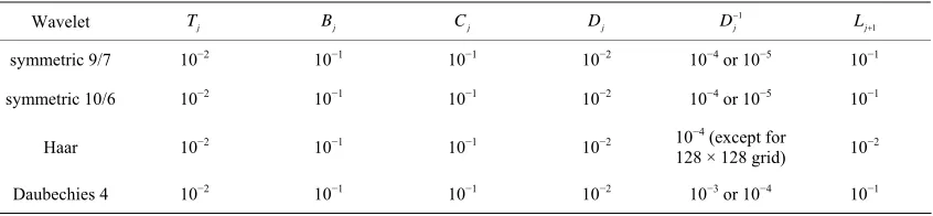
Thresholding values for the three advection-diffusion examples in Section 5.2 are given in Tables 3-5. Note that the thresholding values for 1
j
D (and Lj1 in the
case of parabolic flow (9/7) and recirculant flow (10/6)) for the 9/7 and 10/6 symmetric biorthogonal wavelets depend on the fine grid size and the level of the multigrid method. Similarly, the thresholding values for 1
j
D (and
1 j
L in the case of recirculant flow) for Daubechies 4 wavelets depend on the fine grid size and the level of the multigrid method.
For the advection-diffusion problems with moderately dominant advection, for parabolic flow, for the modified wavelet multigrid method using 9/7 symmetric bior-thogonal wavelets lfil ranges from 2 to 6, depending on
the fine grid size and on the level of the multigrid, and using 10/6 symmetric biorthogonal wavelets, lfil ranges
from 2 to 7. Using the wavelet multigrid method with Haar wavelets, lfil ranges from 2 to 12 and using it with
Daubechies 4 wavelets, lfil ranges from 3 to 6. For
recir-culant flow, lfil ranges from 2 to 5 for 9/7 symmetric
biorthogonal wavelets and from 2 to 4 for 10/6 symmet-ric biorthogonal wavelets, again depending on the fine grid size and on the level. For Haar wavelets, lfil ranges
from 3 to 8, and for Daubechies 4 wavelets, it ranges from 2 to 10. For the problem with skewed vorticity, lfil
ranges from 4 to 7 for 9/7 symmetric biorthogonal wave-lets and from 2 to 6 for 10/6 symmetric biorthogonal wavelets. Using Haar wavelets, lfil ranges from 2 to 10,
and using Daubechies 4 wavelets, it ranges from 4 to 9.
4.3. Storage and Other Computational Issues
The bulk of the remaining computational work occurs in the construction of the intergrid transfer and coarse grid operators. The construction of the intergrid transfer and coarse grid operators each requires two sparse matrix- sparse matrix products and one sparse matrix-sparse ma-trix difference.
[image:6.595.85.511.646.733.2]The storage requirements of the coarse grid and inter-grid transfer operators are minimized by using sparse matrix storage techniques, resulting in storage require-ments of the order of the number of nonzero elerequire-ments in each matrix.
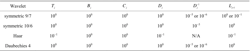
Table 1. Thresholding values for horizontal diffusion example in Section 5.1.
Wavelet Tj Bj Cj Dj
1
j
D Lj1
symmetric 9/7 100 100 100 100 10−5 or 10−6 100 or 10−1
symmetric 10/6 100 100 100 100 10−5 100
Haar 10−1 100 100
Daubechies 4
10−1 N/A 10−1
Table 2. Thresholding values for diagonal diffusion example in
Wavelet
Section 5.1.
j
T Bj Cj Dj
1
j
D Lj1
symmetric 9/7 100 100 100 100 10−5 or 10−6 100 or 10−1
symmetric 10/6 100 100 100 100 10−6 100
Daubechies 4 10− −6
Haar 10−1 10−1 10−1 10−1 N/A 10−1
[image:7.595.85.513.217.320.2]10−1 10−1 10−1 10−1 5 or 10 100
Table 3. Thresholding values for parabolic advection-diffusion example in Section 5.2.
Wavelet Tj Bj Cj Dj
1
j
D Lj1
symmetric 9/7 10− 10− 10−1 10−2 10−4 10
−1 (except for
second level,
2 1
32 × 32 grid)
symmetric 10/6 10 10 10 10 10−2 −1 −1 −2 −4 or 10−5 10−1
Haar 10−2 100 100
Daubechies 4
10−2 10−4 10−2
10−2 100 100 10−2 10−4 or 10−5 10−2
Table 4. Thresholding values for advection-diffusion example with recirculant flow in Section 5.2.
Wavelet Tj Bj Cj Dj
1
j
D Lj1
symmetric 9/7 10−2 10−1 10−1 10−2 10−4 or 10−5 10−1
symmetric 10/6 10−2 10−1 10−1 10−2 10−4 10− −2
Daubechies 4 10− −5 10− −2
1 or 10
Haar 10−2 10−1 10−1 10−2 10−4 10−2
10−2 10−1 10−1 10−2 4 or 10 1 or 10
Table 5. Thresholding values for advection-diffusion example with skewed recirculant flow in Section 5.2.
Wavelet Tj Bj Cj Dj
1
j
D Lj1
symmetric 9/7 10−2 10−1 10−1 10−2 10−4 or 10−5 10−1
symmetric 10/6 10−2 10−1 10−1 10−2 10−4 or 10−5 10−1
Haar 10−2 10−1 10−1 10−2 1 r
128 × 128 grid)
Daubechies 4
0−4 (except fo
10−2
10−2 10−1 10−1 10−2 10−3 or 10−4 10−1
. Numerical Applications
cal results of applying
4096 matrix; and a 128 × 128 grid, leading to a 16384 ×
5
This section describes the numeri
the modified wavelet multigrid method using symmetric biorthogonal wavelets to two diffusion problems with highly oscillatory coefficients and to three advection- diffusion problems with moderately dominant advection. We compare the convergence of the modified wavelet multigrid method using both 9/7 and 10/6 symmetric biorthogonal wavelets with the wavelet multigrid method using both Haar wavelets and Daubechies 4 wavelets. For all problems, numerical results are analyzed using, for the fine grid in the interior, a 32 × 32 grid, leading to a 1024 × 1024 matrix; a 64 × 64 grid, leading to a 4096 ×
16384 matrix. In all problems, the stopping criterion for all multigrid methods is 5
2< 10 k
r , where rk is the
residual obtained from the kth iteration of the method.
5.1. Diffusion Problems
First, we look at the diffusion problem
a x y, u x y,
1 in (15)
, 0 on ,u x y
where We
is the unit square centered at
will examine two cases where
0.5, 0.5 and
0.
[image:7.595.86.510.348.434.2] [image:7.595.88.511.463.561.2]highly oscillatory function:
, 1 0.8sin 10 2
π
,a x y x giving oscillation i the x-direction, and
n
, 1 0.8sin 10 2π
a x y , giv-
ing oscillation along diagonals. Results are examined using both 9/7 and 1
xy
0/6 symmetr
s-Seidel ite ethod is used as the
(16)
where is the unit square centere
ic biorthogonal wavelets. The standard Gaus rative m
smoother.
Tables 6 and 7 compare the average convergence fac-tor per cycle of the modified wavelet multigrid method using symmetric biorthogonal wavelets with that of the wavelet multigrid method. These tables demonstrate re-sults using a fixed coarsest grid size of 8 × 8 for each fine mesh size.
For the diffusion problem with oscillation in x, as well
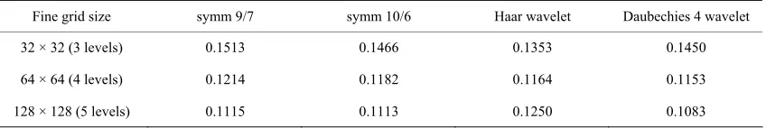
as the diffusion problem with oscillation along diagonals, the convergence of the modified wavelet multigrid method using symmetric biorthogonal wavelets is rela-tively independent of the fine grid size, as it is for the wavelet multigrid method using orthogonal wavelets. Convergence results for the method using both the 9/7 symmetric biorthogonal wavelets and the 10/6 symmetric biorthogonal wavelets are comparable to the results using the orthogonal wavelets for both problems.
5.2. The Advection-Diffusion Problem
Here, we are investigating the problem
0 in
u b u
on ,u f x
d at
0.5, 0.5
and0
thods ar
b . In this problem, difficulties with m
me e encountered due to the of the
nts haracteristics
. W
ultigrid fact that some compone of the solution oscillate along c
[30,31] e apply the wavelet multigrid method to these problems to overcome this difficulty, since application of the wavelet operator preserves the characteristics of the
original problem.
To discretize, we use the standard five-point centered discretization for the diffusion term and a first order up-wind scheme for the advection part of the equation. Al-though using first order upwind introduces artificial dif-fusion into the solution of the order of the mesh size squared, it provides a convenient test of the effectiveness of the modified wavelet multigrid method. Symmetric Gauss-Seidel is used as the smoother in order to ensure that sweeps are performed in the direction of the charac-teristics over the entire flow field. Results shown use
2
10 .
First, we have a comparison of the methods for (16), where
2 1 1
2
, 2
1
b y x xy y and f x
isdefined by
1, if 0, 0, otherwise.x f x
(17)
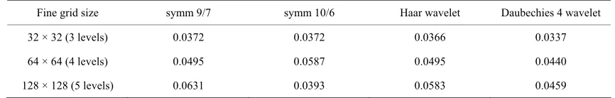
Note that the discontinuous boundary condition will give rise to a boundary layer near the left-hand boundary. Also, the characteristics are parabolic, resulting in flow entering and exiting through the left-hand boundary. For both the modified wavelet multigrid method with sym-metric biorthogonal wavelets and the wavelet multigrid method, convergence appears to be relatively independ-ent of the fine mesh size, as can be seen in Table 8, which compares the average convergence factor per cy-cle using a coarsest grid size of 8 × 8.
In a second example,
4 1 1 2 , 4 1 1 2
b x x y y y x ,
giving recirculant flow (i.e., closed characteristics), and
f x is defined in (17). The modified wavelet
[image:8.595.83.512.562.632.2]multi-grid method using symmetric biorthogonal wavelets and the wavelet multigrid method both have a convergence rate that is relatively independent of the fine grid size. For this problem, the modified wavelet multigrid method
Table 6. Average convergence factor per cy
Fine grid size symm 9/7 symm
cle for diffusion problem with oscillation in x.
10/6 Haar wavelet Daubechies 4 wavelet
32 × 32 (3 levels) 0.1217 0.1137 0.1167 0.1075
64 × 64 (4 levels) 0.1118 0.1087 0.1039 0.1022
128 × 128 (5 levels) 0.1052 0.1177 0.1050 0.1023
ge conver ctor per cycle sion problem diagonals.
[image:8.595.88.512.661.732.2]s sy Ha et Daubechies 4 wavelet
Table 7. Avera gence fa for diffu with oscillation along
Fine grid size ymm 9/7 mm 10/6 ar wavel
32 × 32 (3 levels) 0.1513 0.1466 0.1353 0.1450
64 × 64 (4 levels) 0.1214 0.1182 0.1164 0.1153
Table 8. A nce factor le for the adve ffusion problem arabolic char cs and discon-tinuous bounda
Fine grid size symm 9/7 symm 10/6 Haar wavelet Daubechies 4 wavelet
verage converge ry conditions.
per cyc ction-di with p acteristi
32 × 32 (3 levels) 0.0372 0.0372 0.0366 0.0337
64 × 64 (4 levels) 0.0495 0.0587 0.0495 0.0440
[image:9.595.83.512.220.290.2]128 × 128 (5 levels) 0.0631 0.0393 0.0583 0.0459
Table 9. Ave ce factor cle for the adve lant flow ontinuous
boundary c
s s Ha et Daubechies 4 wavelet
rage convergen per cy ction-diffusion problem with recircu and disc
onditions.
Fine grid size ymm 9/7 ymm 10/6 ar wavel
32 × 32 (3 levels) 0.0488 0.0343 0.0386 0.0370
64 × 64 (4 levels) 0.0525 0.0369 0.0518 0.0584
[image:9.595.84.511.327.396.2]128 × 128 (5 levels) 0.0576 0.0363 0.0482 0.0576
Table 10. Ave ence factor cle for the advec iffusion problem skewed recircu w and
discon-tinuous bo s.
s s Ha et Daubechies 4 wavelet
rage converg per cy tion-d with lant flo
undary condition
Fine grid size ymm 9/7 ymm 10/6 ar wavel
32 × 32 (3 levels) 0.0417 0.0371 0.0384 0.0353
64 × 64 (4 levels) 0.0480 0.0437 0.0403 0.0430
128 × 128 (5 levels) 0.0589 0.0567 0.0551 0.0581
using 10/6 symmetric biorthogonal wavelets outperforms the wavel thod usin Haar wavelet and Dau ts. The are shown in
able 9, which compares the average convergence factor
the modified wavelet multigrid method using symmetric biorthogonal wavelets and the wavelet multi-grid method converge rapidly, with a conv rgence rate that is relatively independent of the fine grid size, as sh
e modificatio elet multig od to use mmetric bior al wavelets ha shown to be effective and utile. The results for the modified wavelet
elet multigrid ently applied in many cases through et multigrid me g both s
bechies 4 wavele results Thsy T
per cycle using a coarsest grid size of 8 × 8.
The final example uses the boundary conditions given by (17), but the advection component has both closed characteristics and a skewed flow, so that it does not line up with the grid. Here,
1 1 11
2 2 22
sin π cos π sin π cos π , cos π sin π cos π sin π ,
b y x y x
y x y x
where
2 2
1 2
2 2
1 2
0.5, 1 0.5, 0.5, 1 0.5.
x x x x
y y y y
Both
e
own in Table 10, which displays the average conver-gence factor per cycle for the modified wavelet multigrid method using both 9/7 and 10/6 symmetric biorthogonal wavelets and for the wavelet multigrid method using both Haar wavelets and Daubechies 4 wavelets. Again, the coarsest grid size for all trials is 8 × 8.
multigrid method using the 9/7 and 10/6 symmetric bior-thogonal wavelets are comparable to those obtained by using the wavelet multigrid method with Haar and Daubechies 4 wavelets. The properties of biorthogonal wavelets should permit the modified wav
6. Conclusion
n of the wav thogon
rid meth s been
method to be effici
the use of compression. The results shown in this paper have demonstrated that it was worthwhile to further ex-plore applying biorthogonal wavelets to the wavelet mul-tigrid method.
REFERENCES
[1] D. De Leon, “A New Wavelet Multigrid Method,”
Jour-nal of ComputatioJour-nal and Applied Mathematics, Vol. 220,
No. 1-2, 2008, pp. 674-675. doi:10.1016/j.cam.2007.09.021
[2] B. Engquist and E. Luo, “The Multigrid Method Based on a Wavelet Transformation and Schur Complement,” Un-published.
[3] D. De Leon, “Wavelet Operators Applied to Multigrid
Methods,” Ph. ngeles, 2000.
[4] W. L. Briggs avelets and
grid,” SIAM Journal on Scientific Computing, Vol. 14,
No. 2, 1993, pp. 506-510. doi:10.1137/0914031 [5] M. Dorobantu and B. Engqu
merical Homogenization,” SIAM
ist, “Wavelet-Based
Journal on Numerical
Analysis, Vol. 35, No. 2, 1998, pp. 540-559.
doi:10.1137/S0036142996298880
[6] B. Engquist and E. Luo, “New Coarse Grid Operators for
, pp Highly Oscillatory Coefficient Elliptic Problems,”
Jour-nal of ComputatioJour-nal Physics, Vol. 129, No. 2, 1996 .
296-306. doi:10.1006/jcph.1996.0251
[7] B. Engquist and E. Luo, “Convergence of a Multigrid Method for Elliptic Equations with Highly Oscillatory Coefficients,” SIAM Journal on Numerical Analysis, Vol.
34, No. 6, 1997, pp. 2254-2273. doi:10.1137/S0036142995289408
[8] N. Neuss, W. Jäger and G. Wittum, “Homogenization and Multigrid,” Computing, Vol. 66, No. 1, 2001, pp. 1-26. doi:10.1007/s006070170036
[9] J. D. Moulton, J. E. Dendy, Jr. and J. M. Hyman, “The Black Box Multigrid Numerical Homogenization Algo-rithm,” Journal of Computational Physics, Vol. 142, No.
1, 1998, pp. 80-108. doi:10.1006/jcph.1998.5911
[10] P. J. Van Fleet, “Discrete Wavelet Transformations: An Elementary Approach with App
science, Hoboken, 2008.
lications,” Wiley-Inter-2/9781118032404 doi:10.100
and Application in Image [11] X. Yang, Y. Shi and B. Yang, “General Framework of the
Construction of Biorthogonal Wavelets Based on Bern stein Bases: Theory Analysis
-Compression,” IET Computer Vision, Vol. 5, No. 1, 2011,
pp. 50-67. doi:10.1049/iet-cvi.2009.0083
[12] W. Sweldens, “The Lifting Scheme: A Construction of Second Generation Wavelets,” SIAM Journal on Mathe-matical Analysis, Vol. 29, No. 2, 1997, pp. 511-546. doi:10.1137/S0036141095289051
[13] D. Taubman and M. Marcellin, “JPEG2000: Image
Com-ms, Theory and
Ill-ystems via Two-Grid pression Fundamentals, Standards and Practice,” The
In-ternational Series in Engineering and Computer Science,
Kluwer Academic, Norwell, 2002.
[14] S. Dahlke and A. Kunoth, “Biorthogonal Wavelets and Multigrid,” In Adaptive Methods: Algorith
Applications, Proceedings of the 9th GAMM Seminar,
Kiel, 1993, pp. 99-119.
[15] L. Cheng, H. Wang and Z. Zhang, “The Solution of Conditioned Symmetric Toeplitz S
and Wavelet Methods,” Computers and Mathematics with Applications, Vol. 46, No. 5-6, 2003, pp. 793-804. doi:10.1016/S0898-1221(03)90142-8
[16] A. P. Reddy and N. M. Bujurke, “Biorthogonal Wavelet Based Algebraic Multigrid Preconditioners for Large Sparse Linear Systems,” Applied Mathematics, Vol. 2, No.
11, 2011, pp. 1378-1381. doi:10.4236/am.2011.211194 [17] W. L. Briggs, S. F. McCormick and V. E. Henson, “A
Multigrid Tutorial,” 2nd Edition, SIAM, Philadelphia, 2000.
doi:10.1137/1.9780898719505
[18] S. McCormick, Ed., “Multigrid Methods,” Frontiers in
Applied Mathematics, SIAM, Philadelphia, 1987.
[19] U. Trottenberg, C. W. Oosterlee and A. Schüller, “Multi-grid,” Academic Press, London, 2001.
[20] J. W. Ruge and K. Stüben, “Algebraic Multigrid,” In:
Multigrid Methods, Frontiers in Applied Mathematics,
SIAM, Philadelphia, 1987, pp. 73-130. doi:10.1137/1.9781611971057.ch4
[21] W. Dahmen and L. Elsner, “Algebraic Multigrid Methods and the Schur Complement,” In: Kiel, Ed., Robust Multi-
An Introduction t 70, GMD, 1999.
Grid Methods, Notes on Numerical Fluid Mechanics, Vol.
23, Vieweg, Braunschweig, 1989, pp. 58-68. [22] K. Stüben, “Algebraic Multigrid (AMG):
with Applications,” Technical Repor
[23] I. Daubechies, “Orthonormal Bases of Compactly Sup-ported Wavelets,” Communications on Pure and Applied
Mathematics, Vol. 41, No. 7, 1988, pp. 909-996.
doi:10.1002/cpa.3160410705
[24] I. Daubechies, “Ten Lectures on Wavelets,” CBMS-NSF
Series in Applied Mathematics, Vol. 61, SIAM,
Philadel-
Com-lied Mathematics, Vol. 45,
phia, 1992.
[25] A. Cohen, I. Daubechies and J.-C. Feauveau, “Biortho- gonal Bases of Compactly Supported Wavelets,”
munications on Pure and App
No. 5, 1992, pp. 485-560. doi:10.1002/cpa.3160450502 [26] D. K. Salkuyeh, “A New Approach to Compute Sparse
Approximate Inverse Factors of a Matrix,” Applied
Mathe-matics and Computation, Vol. 174, No. 2, 2006, pp. 1110-
1121. doi:10.1016/j.amc.2005.06.011
[27] L. Y. Kolotilina and A. Y. Yeremin, “Factorized Sparse Approximate Inverse Preconditioning I. Theory,” SIAM
Journal on Matrix Analysis and Applications, Vol. 14, No.
1, 1993, pp. 45-58. doi:10.1137/0614004
[28] L. Y. Kolotilina and A. Y. Yeremin, “Factorized Sparse Approximate Inverse Preconditioning II: Solution of 3D FE Systems on Massively Parallel Computers,”
Interna-tional Journal of High Speed Computing, Vol. 7, No. 2,
1995, pp. 191-215. doi:10.1142/S0129053395000117 [29] E. Chow and Y. Saad, “Approximate Inverse
Precondi-tioners via Sparse-Sparse Iterations,” SIAM Journal on
Scientific Computing, Vol. 19, No. 3, 1998, pp. 995-1023.
doi:10.1137/S1064827594270415
[30] I. Yavneh, C. H. Venner and A. Brandt, “Fast Multigrid Solution of the Advection Problem with Closed Charac-teristics,” SIAM Journal on Scientific Computing, Vol. 19,
No. 1, 1998, pp. 111-125. doi:10.1137/S1064827596302989
[31] I. Yavneh, “Coarse-Grid Correction for Nonelliptic and Singular Perturbation Problems,” SIAM Journal on
Scien-tific Computing, Vol. 19, No. 5, 1998, pp. 1682-1699.