Data Timed Sending (DTS) Energy Efficient Protocol for Wireless Sensor Networks: Simulation and Testbed Verification

Data Timed Sending (DTS) Energy Efficient Protocol for

Wireless Sensor Networks: Simulation and

Testbed Verification

Konstantin Chomu, Liljana Gavrilovska

Faculty of Electrical Engineering and Information Technologies, Ss Cyril and Methodius University, Skopje, Macedonia Email: chomu@feit.ukim.edu.mk, liljana@feit.ukim.edu.mk

Received June 21,2013; revised July 14, 2013; accepted July 25, 2013

Copyright © 2013 Konstantin Chomu, Liljana Gavrilovska. This is an open access article distributed under the Creative Commons Attribution License, which permits unrestricted use, distribution, and reproduction in any medium, provided the original work is properly cited.

ABSTRACT

The Data Timed Sending (DTS) protocol contributes to the energy savings in Wireless Sensor Networks (WSNs) and prolongs the sensor nodes’ battery lifetime. DTS saves energy by transmitting short packets, without data payload, from the sensor nodes to the base station or the cluster head according to the Time Division Multiple Access (TDMA) sched-uling. Placing the short packets into appropriate slots and subslots in the TDMA frames transfers the information about the measured values and node identity. This paper presents the proof of concept of the proposed DTS protocol and pro-vides verification of the energy savings using the QualNet® _{communication simulation platform (QualNet) and the}

SunTM _{Small Programmable Object Technology (Sun SPOT) testbed platform (for single hop and multi hop scenarios).}

The simulations and the testbed measurements confirm that the DTS protocol can provide energy savings up to 30% when compared with the IEEE 802.15.4 standard in unslotted Carrier Sense Multiple Access with Collision Avoidance (CSMA-CA) mode at 2.4 GHz frequency band.

Keywords: Data Timed Sending; Energy Efficiency; Wireless Sensor Networks

1. Introduction

The Wireless Sensor Networks (WSNs) have become an important tool for gathering information in all areas of the human life. A WSN is a network made of small size and low-power sensor nodes with capabilities to collect, process, and wirelessly transmit various types of data. The WSN platforms introduce different routings [1-3], power management [4-9], and synchronization protocols [10-15]. The specific WSN requirements contribute to the development and implementation of various operat- ing systems [16] and applications [17]. The possible ap- plications cover a wide range of areas, such as environ- mental monitoring, medical care, smart homes, robot controlling, security, public safety, surveillance, com- mercial applications, tracking, identification, personal- ization, etc.

A typical WSN consists of spatially distributed auto- nomous battery powered sensor nodes, which sense and cooperatively pass their data to a base station directly (single hop) or through the intermediate nodes (multi hop). Changing or recharging the batteries on remote

nodes is a difficult, time-consuming and expensive task. It is very important for the WSNs to reduce the amount of energy consumption in each node, which in turn ex-tends the network lifetime and reduces the number of the necessary interventions. Some energy saving solutions reduce the packet loss ratio and the length of a packet’s route by exploiting energy aware routing [6,7,9,18,19], whereas others are oriented towards energy harvesting methods [20-22]. The energy aware routing improves the energy conservation in conditions of congestion or link failure.

(CSMA-CA) protocol according to the IEEE 802.15.4- 2006 standard. The simulations are performed on a Qual Net simulator, and the testbed implementation is realized

on a SunTM _{Small Programmable Object Technology}

(Sun SPOT) WSN testbed platform. This paper is organ- ized as follows. The second section describes the DTS protocol. The third section gives the power consumption analysis. The fourth section presents the simulation sce- narios and results. The fifth section describes the Sun SPOT testbed platform, whereas the sixth section pro- vides the results of the energy consumption comparison. The seventh section gives the conclusions.

2. DTS Protocol

The DTS is TDMA based protocol. It can support single hop and multi hop topologies. When a DTS-enabled WSN uses single hop topology, it is organized as a star network where every remote sensor node sends packets directly to the base station. When a DTS-enabled WSN uses multi hop topology, it is organized as a cluster net-work where nodes are grouped in clusters. Each cluster has one cluster-head node. In the cluster network every remote sensor node sends packets to its cluster-head, which acts as an intermediate node to the base station.

2.1. DTS in Single Hop Topology

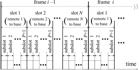
In a single hop scenario the time is organized in frames, where each frame is divided in N slots, and each slot is divided in P + 1 subslots, as shown in Figure 1. The pa-rameter N is the number of the remote sensor nodes as-sociated with the base station and P is the number of the possible values of the measured phenomenon. Each node has dedicated slot and each measured value has dedicated subslot. During each frame, each node sends one short packet (without data payload) about the measured value during the previous frame. The node transmits short packet in the slot and the subslot that correspond to the node’s ordinal number and the measured value, respec-tively. The base station can recognize which node has sent the short packet and what is the measured value only by its positioning within the frame. The requirements of

time

frame i–1 frame i

slot 1 slot 2 slot N slot 1

subs

lot

1

su

bs

lo

t

2

su

bs

lo

t

P

+1

su

bs

lo

t

1

subs

lot

2

subs

lot

P

+1

su

bs

lo

t

1

subs

lot

2

subs

lot

P

+1

su

bs

lo

t

1

subs

lot

2

subs

lot

P

+1

remote 2 to base

( )

( )

( )

remote N

to base

( )

Figure 1. Time division scheme for single hop DTS.

a particular WSN application determine the length of the frames and the number of the slots and subslots. The DTS protocol synchronizes the nodes with the base sta-tion [24]. The synchronizasta-tion mechanism works by broadcasting the resynchronization packets from the base station in regular resynchronization intervals. The dura-tion of the resynchronizadura-tion interval depends on the application requirements.

The duration of the short packet as well as the duration of the resynchronization packet must be less than the duration of one subslot. The minimum packet’s size de-pends on the hardware characteristics of the node’s radio (8 bytes for the Sun SPOT’s radio chip). The size of the short and the resynchronization packets is usually equal to the minimum packet’s size allowed by the node’s ra-dio chip in order to maximize the energy savings (shorter packet keeps the radio less time switched on).

The sensor nodes are in sleeping mode most of the time and they wake up only to send the short packet to the base station, to take new measurement or to receive a resynchronization packet. The base station broadcasts the resynchronization packet in a subslot determined by the resynchronization interval. Therefore, the number of the subslots is P + 1.

The statistical synchronization protocols [10,11,14], can achieve a synchronization error of less than 10 mi-croseconds. With such small errors, a 30 second long slot can contain 60,000 subslots where each subslot is wide enough to accept a 15 byte packet at 250 kb/s bit rate along with two error margins. It allows using the single subslot not just for one value of one measured pheno- menon, but for a combination of values of several phe- nomena (e.g. temperature, air pressure, and humidity). In cases of environmental monitoring, the sensor should collect data with rate at least equal to changes of envi-ronmental conditions noticeable for humans or other liv-ing organisms (usually once in 5 to 10 minutes) [25]. Due to limited number of packet transmissions and syn-chronization constraints [24], the DTS protocol is suit-able for WSN applications that do not demand extremely high bit rates.

2.2. DTS in Multi Hop Topology

In a multi hop scenario the time is organized in frames, where each frame is divided in two subframes, i.e., in subframe A and subframe B, as shown in Figure 2. The subframe A covers the time when the remote sensor nodes send packets to their corresponding cluster-head node, and the subframe B covers the time when the clus- ter-head nodes send packets to the base station.

time

frame i–1 frame i

subframe A subframe B subframe A

remote to cluster-head

( )

cluster-head

( )

cluster-head to base station

( )

Figure 2. Time division scheme for multi hop DTS.

time

subframe A (common for all clusters) subframe B slot 1 slot 2 slot R

su bs lo t 1 su bs lo t 2 su bs lo t M +1 su bs lo t 1 su bs lo t 2 su bs lo t M +1 su bs lo t 1 su bs lo t 2 su bs lo t M +1

remote 1 to cluster-head

( )

( )

( )

Figure 3. Time division scheme for subframe A (each clus-ter has R remote sensor nodes).

associated with one cluster-head node, and M is the number of the possible values of the measured phe-nomenon. Each remote sensor node has dedicated slot and each measured value has dedicated subslot. During each subframe A, each remote sensor node sends one short packet (without data payload) with information about the measured value during the previous frame. The remote sensor node transmits short packet in the slot and the subslot that correspond to the remote sensor node’s ordinal number and the measured value, respectively. The cluster-head node can recognize which node has sent the short packet and what the measured value is only by its positioning within the subframe A. All clusters are far apart from each other or they use different frequency channels, so the subframe A is common for all cluster- heads.

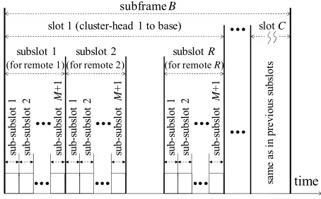
The subframe B is divided in C slots, each slot is di-vided in R subslots, and each subslot is divided in M+1 sub-subslots, as shown in Figure 4. The required diapa-son and granulation of the measured phenomenon deter-mines the number of the sub-subslots. The parameter C is the number of the cluster-head nodes associated with the base station, R is the number of the remote sensor nodes associated with one cluster-head node, and M is the number of the possible values of the measured phe-nomenon. Each cluster-head node has dedicated slot, each remote sensor node has dedicated subslot, and each measured value has dedicated sub-subslot. During each subframe B, each cluster-head node sends R short packets (without data payload) about the measured value during the previous frame. The cluster-head node transmits short packet in the slot, subslot, and the sub-subslot that cor-respond to the cluster-head node’s ordinal number, re-mote sensor node’s ordinal number, and the measured

time

subframe B

slot 1 (cluster-head 1 to base) slot C

su b-su bs lo t 1 su b-su bs lo t 2 su b-su bs lo t M +1 sa m e a s i n pr evi ous s ubs lo ts

subslot 1 subslot 2 subslot R

su b-su bs lo t 1 su b-su bs lo t 2 su b-su bs lo t M +1 su b-su bs lo t 1 su b-su bs lo t 2 su b-su bs lo t M +1

(for remote 1) (for remote 2) (for remote R)

Figure 4. Time division scheme for subframe B.

value, respectively. The base station can recognize which cluster-head node has sent the short packet, which remote sensor node represents that short packet, and what the measured value is only by packet’s position within the subframe B.

The synchronization mechanism works by broadcast-ing the resynchronization packets from the base station in regular resynchronization intervals.

The remote sensor nodes are in sleeping mode most of the time and they wake up only to send the short packet to the cluster-head node, to take new measurement or to receive a resynchronization packet. The base station broad- casts the resynchronization packet in a subslot or sub- subslot determined by the resynchronization interval. Therefore, the number of the subslots and sub-subslots is M + 1.

The DTS protocol is convenient for static rather than ad hoc network scenarios since the software reflects the topology and need to be upgrade if the topology changes.

3. Power Consumption

The characteristics of the sensor nodes have a significant impact on its power consumption. The usual design ap-proach for ultra low-powered devices, such as sensor nodes, is to minimize the average current draw by spending as much time as possible in a low-power con-sumption mode so-called sleep mode. In the active period, the device intensively draws current from its battery. After the active period, the device returns into a sleeping mode.

3.1. Distribution of Power Consumption

The sensor node comprises four entities that are major power consumers, i.e., the radio, the microcontroller, the interface circuitry and the software running on the mi-crocontroller. They are briefly described in the following text.

 Radio—the WSN nodes are devices with limited

that cannot receive and transmit simultaneously. The transmitting current draws are at a scale of tens of milliamps, whereas the low-power mode current draw is at a scale of microamps [4]. Since the radio usage consumes the majority of the node energy [26], the development of low energy consumption Medium Access Control (MAC) protocols is of great impor- tance for WSNs.

 Microcontrollers—microcontrollers comprise a Cen-

tral Processor Unit (CPU), timers, Universal Asyn- chronous Receivers Transmitters (UARTs), inputs, outputs, etc. Power consumption of a CPU depends on its implementation, i.e., on the application de- mands. The current draw in active mode exceeds hundred milliamps, whereas in a low-power mode it is at a scale of microamps.

 Interface Circuitry—this circuit depends on the

ap-plication. It includes light indicators, external analog or digital inputs and outputs, relays, etc. The current draw varies in a range from tens to hundred of milli-amps [4]. The microcontroller needs to be awake to change the state of an output, but it can turn to sleep leaving an output device powered on.

 Software—the software can manage the switching on

and off of the processes. The software can be de- signed by the user as an application or by the manu- facturer as an operating system. The overall software is designed to minimize the power consumption.

3.2. Power Consumption of IEEE 802.15.4 with 2.4 GHz Unslotted CSMA-CA

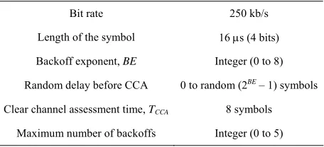
The IEEE 802.15.4 standard defines a symbol as the smallest operational time unit. Table 1 lists the parame-ters of the IEEE 802.15.4 unslotted CSMA-CA in the 2.4 GHz band [27].

When a node needs to transmit a data packet, it waits for a random time and then performs Clear Channel As-sessment (CCA), i.e., hears if the channel is idle or busy. If the channel is idle, the node transmits the data packet. If the channel is busy, the node backs off, i.e., waits for another random time before it performs the next CCA. The node repeats this procedure, but if the algorithm ex-

Table 1. Parameters of IEEE 802.15.4 unslotted CSMA-CA at 2.4 GHz.

Bit rate 250 kb/s

Length of the symbol 16 s (4 bits)

Backoff exponent, BE Integer (0 to 8)

Random delay before CCA 0 to random (2BE _{– 1) symbols}

Clear channel assessment time, TCCA 8 symbols

Maximum number of backoffs Integer (0 to 5)

ceeds the maximum allowed number of backoffs, then the transmission is canceled [27]. The average number of backoffs NAvBack is derived from the analysis based on

[28].

Probability that a node transmits in a CCA period, ATrCCA is given with:

iod FixTimePer

AvChOccup

T

T

A



where TAvChOccup is average channel occupation time in a

fixed time period, TFixTimePeriod. The designer defines both

TAvChOccup and TFixTimePeriod.

Probability ACC that a channel is idle after the first

backoff interval, for network with NS sensor nodes, is

given with:





1 NS

CC TrCCA

A  A  . (2)

According to the IEEE 802.15.4, the overall backoff time can be comprised of up to five backoff intervals plus associated CCA periods. In the case of maximum five backoff intervals [27], the probability of transmis-sion, ATR is:















1

1

1 n

n CC CC

TR A A

A

Then, the average number of backoffs, NAvBack

be-comes:











 

5

1

1 1

n

n

CC CC

AvBack nA A

N . (4)

The unslotted CSMA-CA average receiver power consumption, PUnAvRXis:





   



   



SndUn

ACK CCA AvBack StRX

AvBack

T

T T N T N

P

P_{UnAvRX RX} 1

(5) where PRX is active receiver power consumption, TStRX is

the receiver start-up time, TCCA is time for performing

CCA, TACK is acknowledgment packet duration (if

ac-knowledgment is required), and TSndUn is a interval in

which node sends one data packet.

The unslotted CSMA-CA average transmitter power consumption, PUnAvTX is defined as:

   



 



SndUn DAT StTX

T T T P

P_{UnAvTX TX} (6)

where PTX is active transmitter power consumption, TStTX

is the transmitter start-up time and TDAT is the duration of

the data packet.

3.3. Power Consumption of DTS

packets. DTS requires synchronization among the nodes and the base station. Base station broadcast resynchroni-zation packets in order to achieve the synchroniresynchroni-zation. The clock of the base station is designated as a reference clock. The base station broadcasts the resynchronization packet every time its resynchronization timer reaches the value of the resynchronization interval, TRI. Then, the

base station sets its resynchronization timer back to the zero value and starts a new counting. All nodes simulta-neously receive the resynchronization packets and syn-chronize their timers with the base station timer. To overcome the uncertainty between the node’s local no-tion of time and that of the base stano-tion, the node turns on its receiver shortly (i.e. TGuard) before its timer reaches

the TRI value. Longer values of the resynchronization

interval TRI result in greater drift accumulation from the

clock frequency errors.

The DTS average receiver power consumption,

PDTSAvRX is only a consequence of the reception of the

resynchronization packet and is defined as:

   



  



RI

RSP Guard StRX

T T T T P

P_{DTSAvRX RX} (7)

where PRX and TStRX are active receiver power

consump-tion and receiver start-up time respectively, and TRSP is

the duration of the resynchronization packet.

The DTS average transmitter power consumption, PDTSAvTX is defined as:

   



 



SndDTS DTS StTX

T T T P

PDTSAvTX TX (8)

where PTX is active transmitter power consumption, TStTX

is the transmitter start-up time, TDTS is the duration of

short DTS packet and TSndDTS is frame duration in which

the node sends one short DTS packet.

3.4. Energy Consumption Challenges

The rapid and sudden changes of the current draw at the WSN nodes impose serious difficulties in their energy consumption monitoring. The consumed energy En in

time interval T that starts at t = t0 and ends at t = t0 + T is

given with:

   

0

d

b

t T

n b

t

E u t i t





_

where ub(t) is the voltage of the battery and ib(t) is the

battery current draw. Battery voltage does not change drastically although the current can vary from microamps to tens or hundreds of milliamps (more than three orders of magnitude) in the scale of microseconds [29]. Rapid change of the current draw is mostly a consequence of the occasionally awakening of the node to take a reading

or send a packet and sleeping on the remainder of the time. The current variation causes variation of the con-sumed energy in the scale of microseconds. Simple ap-proximations of nodal energy consumption derived from estimates of duty cycle and receiving/transmitting rates (5)-(8) do not capture entirely the low-level system power profile of the WSNs [29]. A node can exhibit a bewildering array of power profiles depending on its application profile. Another problem is short-duration power spikes during periods of brief activities of the op-erating system or background processes. Additional in-consistency of the current draw is due to the temperature variation, which affects the current leakage [29]. These are the motivations to implement a given WSN protocol on a real platform in order to discover its true perform-ances.

4. Simulation Scenario

The proof of concept for the energy efficiency of the proposed DTS protocol was confirmed with simulation setup performed with QualNet. QualNet can model sce-narios for large number of nodes by taking advantage of the latest hardware and parallel computing techniques. It includes advanced models for the wireless environment to enable more accurate modeling of real-world wireless networks. This section presents the simulation result used for comparison of energy consumption of DTS with IEEE 802.15.4 unslotted CSMA-CA protocols.

4.1. Simulation Architecture and Scenario

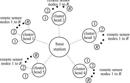
Simulation scenarios include cases for different number of remote sensor nodes grouped in clusters, as shown in

Figure 5. Remote sensor nodes from one cluster send

packets to their cluster-head node, which in turn sends packets to the base station. Tables 2 and 3 list the pa-rameters of the IEEE 802.15.4 and DTS.

The number of the clusters is 5. In this scenario, the clusters are sufficiently distant from each other to ex-

base

cluster head 1

cluster head 2

cluster head 3

cluster

head 5 cluster_{head 4}

station 1

2 R

1

2 R

1 2

R

1 2

R

1 2

R

remote sensor nodes 1 to R

remote sensor nodes 1 to R

remote sensor nodes 1 to R

remote sensor nodes 1 to R

remote sensor nodes 1 to R

Table 2. Parameters of QualNet simulation scenario for IEEE 802.15.4 unslotted CSMA-CA.

Total number of remote sensor nodes 10, 20, … to 100

Time interval to perform readings

and send one standard packet 20 min

PHY layer protocol IEEE 802.15.4

MAC layer protocol IEEE 802.15.4

Routing protocol ZigBee (AODV)

Observed statistics

 average energy consumption per remote node

 standard deviation of average energy consumption per remote node

Table 3. Parameters of QualNet simulation scenario for DTS protocol.

Total number of remote sensor nodes 10, 20, … to 100

Time interval to perform readings

and send one short DTS packet 20 min

PHY layer protocol DTS

MAC layer protocol DTS

Routing protocol DTS

Observed statistics

 average energy consumption per remote node

 standard deviation of average energy consumption per remote node

clude interference. (In reality, another way to exclude interference is to allocate different frequency channels to clusters.) Connection between each remote sensor node and the base station is multi hop. Simulations are re- peated 10 times, starting with a total of 10 remote sensor nodes (2 remote nodes per one cluster-head), and ending with a total of 100 remote sensor nodes (20 remote nodes per one cluster-head). Each remote sensor node takes measurement readings and sends a packet once in 20 minutes (which corresponds to the realistic environ- mental monitoring scenarios, e.g. air temperature).

The simulation setup was used to confirm the advan- tages of the DTS compared with the IEEE 802.15.4. QualNet simulator runs scenario with IEEE 802.15.4 unslotted CSMA-CA protocol on PHY and MAC layers and utilizes ZigBee (variation of Ad hoc On-Demand Distance Vector (AODV)) as routing protocol. In DTS case, the QualNet simulator runs scenario with DTS pro- tocol on PHY, MAC, and routing layers.

4.2. Simulation Results

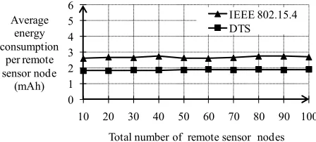
The average energy consumption per remote sensor node shows the energy efficiency of both protocols. Figures 6 and 7 give the average energy consumption per remote

0 1 2 3 4 5 6

10 20 30 40 50 60 70 80 90 100 Average

energy consumption

per remote sensor node

(mAh)

Total number of remote sensor nodes IEEE 802.15.4 DTS

Figure 6. Average energy consumption comparison of DTS with IEEE 802.15.4 (QualNet simulation).

0 0.2 0.4 0.6 0.8 1 1.2

10 20 30 40 50 60 70 80 90 100 Standard

deviation of average

energy consuption

per remote sensor node

(mAh)

Total number of remote sensor nodes IEEE 802.15.4 DTS

Figure 7. Standard deviation of average energy consump-tion comparison of DTS with IEEE 802.15.4 (QualNet simu-lation).

sensor node and the standard deviation of the average energy consumption per node, respectively, for 10, 20, … to 100 total number of remote sensor nodes. Table 4 summarizes the simulation results.

Simulations show that DTS protocol consumes ap- proximately 30% less energy than IEEE 802.15.4 unslot- ted CSMA-CA protocol, and energy savings do not de- pend on the total number of remote sensor nodes. Simu- lations also show that DTS protocol has constant and lower standard deviation of the energy consumption than IEEE 802.15.4 unslotted CSMA-CA, whose standard deviation of the energy consumption increases with lar-ger number of remote sensor nodes.

For IEEE 802.15.4 scenario, the standard deviation of the energy consumption per remote node experiences approximately linear growth as total number of remote sensor nodes increase. This is due to increase in packet collisions and medium occupancy as total number of remote sensor nodes increase. In such conditions some remote nodes do not receive acknowledgement packet and perform retransmission (spend more energy than average), whereas other remote nodes detect busy chan-nel consequently several times and disclaim transmission (spend less energy than average). For DTS scenario, each transmission has dedicated time slot, so remote nodes neither retransmit packets nor disclaim transmission of the packets.

5. Testbed Platform

Table 4. Results from QualNet simulation.

Energy savings achieved by

DTS over IEEE 802.15.4 30%

Standard deviation of energy consumption with DTS

≈ 0.2 mAh (approximately constant) Standard deviation of energy

consumption with IEEE 802.15.4

approximately linear growth from 0.2 mAh (for 10 remote sensor nodes) to 0.8 mAh (for 100 remote sensor nodes)

consumption between the DTS and IEEE 802.15.4 un-slotted CSMA-CA and to prove the energy efficiency of the DTS in realistic environment. The testbed works in a laboratory indoor environment. The testbed WSN appli-cation measures the air temperature and luminosity. This section presents the testbed scenarios and results.

5.1. Testbed Architecture and Scenario

The testbed consists of 8 Sun SPOTs that act as remote sensor nodes, 2 Sun SPOTs that act as cluster-head nodes, and one base station attached to the laptop host computer via Universal Serial Bus (USB) cable, as shown in

Fig-ure 8. The base station serves as a gateway to the host

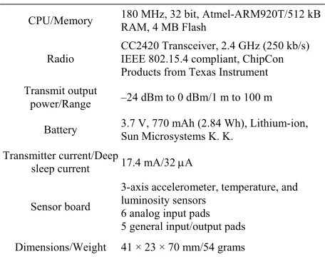
computer. The cluster-head Sun SPOTs are labeled as cluster-head nodes 1 and 2. Remote Sun SPOTs are la-beled as remote nodes 1, 2, … to 8. The remote nodes were placed at distances less than 10 m from their corre-sponding cluster-heads, and the cluster-heads were placed at distances less than 10 m from the base station. The Sun SPOTs are Sun Microsystems-2008 model. Ta-

ble 5 lists Sun SPOTs’ hardware characteristics [30- 33].

Remote nodes 1 to 4 are connected to the cluster-head node 1, and remote nodes 5 to 8 are connected to the cluster-head node 2.

Communication between remote nodes 1 to 4 and the cluster-head 1 is set up on IEEE 802.15.4 radio channel 11, and communication between remote nodes 5 to 8 and the cluster-head 2 is set up on IEEE 802.15.4 radio channel 12. Communication between cluster head nodes 1, 2, and the base station is on IEEE 802.15.4 radio channel 25. When testbed works with DTS protocol, the base station sends resynchronization packets at IEEE 802.15.4 radio channel 25.

During the IEEE 802.15.4 measurement, the remote sensor nodes use an energy saving sleep mode and wake up once in every 1200 s to take temperature and luminos-ity measurement and to send data packet to the base sta-tion via their corresponding cluster-head nodes. The PHY and MAC layers works with IEEE 802.15.4 unslot-ted CSMA-CA standard, and the routing protocol is 6LoWPAN (IPv6 compatible Low power Wireless Per-sonal Area Networks). In terms of energy efficiency, 6LoWPAN and ZigBee are very similar, i.e., the both are designed for small low-power devices with limited proc-essing capabilities. After measuring and sending the

host computer stationbase

remote node 1 remote node 2

remote node 3

remote node 4

cluster-head node 1

remote node 8 remote

node 5 remote node 6

remote node 7

cluster-head node 2

Figure 8. Cluster topology architecture for Sun SPOT test-bed platform.

Table 5. Sun SPOT Hardware Characteristics.

CPU/Memory 180 MHz, 32 bit, Atmel-ARM920T/512 kB _{RAM, 4 MB Flash}

Radio

CC2420 Transceiver, 2.4 GHz (250 kb/s) IEEE 802.15.4 compliant, ChipCon Products from Texas Instrument Transmit output

power/Range –24 dBm to 0 dBm/1 m to 100 m

Battery 3.7 V, 770 mAh (2.84 Wh), Lithium-ion, _{Sun Microsystems K. K.}

Transmitter current/Deep

sleep current 17.4 mA/32 A

Sensor board

3-axis accelerometer, temperature, and luminosity sensors

6 analog input pads 5 general input/output pads

Dimensions/Weight 41 × 23 × 70 mm/54 grams

packet, the sensor node is going back to sleep mode. During the DTS measurements, the remote sensor nodes use an energy saving sleep mode and wake up once in every 20 minutes to take temperature and lumi- nosity measurement and to send short DTS packet to their corresponding cluster-head nodes. After the clus- ter-heads receive short DTS packets from all remote nodes in their cluster, they begin to send short DTS packets to the base station. All remote and cluster-head nodes also wake up once in every 60 minutes to receive the short resynchronization DTS packet. In this mode, DTS protocol covers the PHY layer, MAC layer, and the routing procedure.

Tables 6 and 7 list the parameters of the IEEE 802.

15.4 and DTS scenarios. Table 8 lists DTS TDMA

scheduling of the remote and cluster-head nodes. The terms in Table 8 are consistent with the terms described

in Figures 2-4.

Table 6. Parameters of Sun SPOT testbed scenario for IEEE 802.15.4 unslotted CSMA-CA.

Total number of remote sensor nodes 8

Time interval to perform readings

and send one standard packet 20 min Range/resolution of

measured temperature (90 possible values) –39˚C to 50˚C /1˚C Range/resolution of

measured luminosity

0 lx to 1000 lx/100 lx (11 possible values)

Combinations of measured phenomena 990

PHY layer protocol IEEE 802.15.4

MAC layer protocol IEEE 802.15.4

Routing protocol 6 Low PAN

Observed statistics battery voltage reading every _{5 minutes}

Table 7. Parameters of Sun SPOT testbed scenario for DTS protocol.

Total number of remote sensor nodes 8

Time interval to perform readings and

send one standard packet 20 min

Range/resolution of measured temperature _{(90 possible values)} –39˚C to 50˚C /1˚C

Range/resolution of measured luminosity 0 lx to 1000 lx/100 lx_{(11 possible values)}

Combinations of measured phenomena 990

PHY layer protocol DTS

MAC layer protocol DTS

Routing protocol DTS

Observed statistics battery voltage reading _{every 5 minutes}

Table 8. DTS TDMA values for Sun SPOT testbed.

Duration of subframe A 400 s

Number of slots in frame A/Duration 4/100 s

Number of subslots in one slot in frame A/Duration 1000/100 ms

Duration of subframe B 800 s

Number of slots in frame B/Duration 2/400 s

Number of subslots in one slot in frame B/Duration 4/100 s

Number of sub-subslots in one

subslot in frame B/Duration 1000/100 ms

providing an evaluation of the energy consumption. The most significant point of the curve is the moment when the voltage drops to a critical value at which the remote Sun SPOT stops to work.

Sun SPOTS are manufactured with embedded IEEE 802.15.4 unslotted CSMA-CA (PHY and MAC layers)

and with embedded 6LoWPAN routing protocol. But, for the DTS evaluation, the existing network software is re-placed with custom made software in order to implement the DTS functionalities.

5.2. Testbed Results

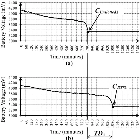
The discharge curves for each remote Sun SPOT pro-vides evaluation of its energy consumption. Figures 9(a) and (b) show the discharge curve of the remote Sun SPOT 1 when it works with the IEEE 802.15.4 unslotted CSMA-CA and DTS protocol, respectively. The critical points CUnslotted1 and CDTS1 mark the time and the battery

voltage level of the remote Sun SPOT 1, when it stops to work with the IEEE 802.15.4 unslotted CSMA-CA and DTS protocol, respectively. The flat lines give the last recorded voltage levels in remote Sun SPOT 1 flash memory before its battery is fully discharged. The time difference between the critical points CDTS1 and CUnslotted1,

TD1, gives the quantity of the energy savings. For the

remote Sun SPOT 1, the time difference is 27%, which indicates that the DTS achieves 27% energy savings when compared with the 2.4 GHz, unslotted CSMA-CA IEEE 802.15.4. The remote Sun SPOTs 2 to 8 have simi- lar discharge curves and Figure 10 shows their energy savings. Table 9 summarizes the results from the testbed platform.

The difference among the discharging times of remote Sun SPOTs 1 to 8, when they are working with the IEEE 802.15.4 or DTS, is due to the different individual bat-tery characteristic, hardware imperfection and other ex-ternal influences. However, it is evident that DTS pro-

3000 3200 3400 3600 3800 4000 4200 4400

0 ₆₀

120 180 240 300 360 420 480 540 600 660 720 780 840 900 960 _{1020 1080 1140 1200 1260 1320 1380}

B

atte

ry

V

olta

ge

(m

V

)

Time (minutes)

(a)

CUnslotted1

3000 3200 3400 3600 3800 4000 4200 4400

0 ₆₀

120 180 240 300 360 420 480 540 600 660 720 780 840 900 960 ₁₀20 ₁₀80 ₁₁40 ₁₂00 ₁₂60 ₁₃20 ₁₃80

B

atte

ry

V

ol

ta

ge

(m

V

)

Time (minutes)

(b)

CDTS1

TD1

0 5 10 15 20 25 30 35

1 2 3 4 5 6 7 8

E

ner

gy s

av

ing

s of

D

T

S

ove

r

IE

E

E

802.

15

.4

(%

)

Remote Sun SPOT's ID

Figure 10. Energy savings of DTS protocol over IEEE 802.15.4 for remote Sun SPOTs 1 to 8.

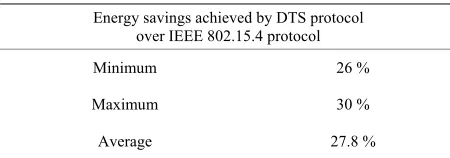
Table 9. Results from Sun SPOT testbed platform.

Energy savings achieved by DTS protocol over IEEE 802.15.4 protocol

Minimum 26 %

Maximum 30 %

Average 27.8 %

vides energy savings approximately around 30%.

6. Conclusion

This paper presents proof of concept for DTS energy efficient protocol and gives a QualNet simulation and Sun SPOT testbed verification for significant energy savings of 30% achieved when compared with IEEE 802.15.4 unslotted CSMA-CA. DTS protocol uses TDMA approach for communication combined with short packets without data payload. The simulation and the testbed results are consistent and proof the energy efficiency of the DTS in WSNs.

7. Acknowledgements

This work was supported in part by the European Com-mission FP7 ProSense project under Grant agreement no. 205494.

REFERENCES

[1] S. K. Singh, M. P. Singh and D. K. Singh, “Routing Pro-tocols in Wireless Sensor Networks—A Survey,” Inter- national Journal of Computer Science & Engineering Survey, Vol. 1, No. 2, 2010, pp. 63-83.

doi:10.5121/ijcses.2010.1206

[2] L. J. G. Villalba, A. L. S. Orozco, A. T. Cabrera and C. J. B. Abbas, “Routing Protocol in Wireless Sensor Net- works,” Sensors, Vol. 9, No. 11, 2009, pp. 8399-8421. doi:10.3390/s91108399

[3] Y. Al-Obaisat and R. Braun, “On Wireless Sensor Net- works: Architectures, Protocols, Applications, and Man-

agement,” Proceedings of theAusWireless 2006 Confer- ence, Sydney, 13-16 March 2006, pp. 1-11.

[4] A. Norouzi and A. Sertbas, “An Integrated Survey in Efficient Energy Management for WSN using Architec- ture Approach,” International Journal of Advanced Net- working and Applications, Vol. 3, No. 1, 2011, pp. 968- 977.

[5] M. D. Francesco, G. Anastasi, M. Conti, S. K. Das and V. Neri, “Reliability and Energy-Efficiency in IEEE 802.15. 4/Zigbee Sensor Networks: An Adaptive and Cross-Layer Approach,” Selected Areas in Communications, Vol. 29, No. 8, 2011, pp. 1508-1524.

doi:10.1109/JSAC.2011.110902

[6] S. K. Singh, M. P. Singh and D. K. Singh, “Energy-Effi- cient Homogeneous Clustering Algorithm for Wireless Sensor Network,” International Journal of Wireless & Mobile Networks, Vol. 2, No. 3, 2010, pp. 49-61. doi:10.5121/ijwmn.2010.2304

[7] M. Liu, J. Cao, G. Chen and X. Wang, “An Energy- Aware Routing Protocol in Wireless Sensor Networks,” Sensors, Vol. 9, No. 1, 2009, pp. 445-462.

doi:10.3390/s90100445

[8] H. Abusaimeh and S. H. Yang, “Dynamic Cluster Head for Lifetime Efficiency in WSN,” International journal of Automation and Computing, Vol. 6, No. 1, 2009, pp. 48- 54. doi:10.1007/s11633-009-0048-0

[9] A. G. A. Elrahim, H. A. Elsayed, S. E. Ramly and M. M. Ibrahim, “An Energy Aware WSN Geographic Routing Protocol,” Universal Journal of Computer Science and Engineering Technology, Vol. 1, No. 2, 2010, pp. 105-111. [10] C. Lenzen, T. Locher and R. Wattenhofer, “Tight Bounds

for Clock Synchronization,” Journal of the ACM (JACM), Vol. 57, No. 2, 2010, Article No. 8.

doi:10.1145/1667053.1667057

[11] C. Lenzen, P. Sommer and R. Wattenhofer, “Optimal Clock Synchronization in Networks,” Proceedings of the 7th ACM Conference on Embedded Networked Sensor Systems, Berkeley, 4-6 November 2009, pp. 225-238.

doi:10.1145/1644038.1644061

[12] P. Sommer and R. Wattenhofer, “Gradient Clock Syn-chronization in Wireless Sensor Networks,” Proceedings of the 8th ACM/IEEE International Conference on In-formation Processing in Sensor Network 2009, San Fran- cisco, 13-16 April 2009, pp. 37-48.

[13] S. Ganeriwal, R. Kumar and M. B. Srivastava, “Tim-ing-Sync Protocol for Sensor Networks,” Proceedings of the 1st International Conference on Embedded Net- worked Sensor Systems, Los Angeles, 5-7 November 2003, pp. 138-149. doi:10.1145/958491.958508

[14] M. Maroti, B. K. G. Simon and A. Ledeczi, “The Flood-ing Time Synchronization Protocol,” Proceedings of the 2nd International Conference on Embedded Networked Sensor Systems, Baltimore, 3-5 November 2004, pp. 39- 49. doi:10.1145/1031495.1031501

[16] M. O. Farooq and T. Kunz, “Operating Systems for Wireless Sensor Networks: A Survey,” Sensors, Vol. 11, No. 6, 2011, pp. 5900-5930. doi:10.3390/s110605900 [17] C. F. Garcia-Hernandez, P. H. Ibarguengoytia, J.

Gar-cia-Hernandez and J. A. Perez-Diaz, “Wireless Sensor Networks: A Survey,” International Journal of Advanced Networking and Applications (IJANA), Vol. 7, No. 3, 2007, pp. 264-273.

[18] K. Padmanabhan and P. Kamalakkannan, “A Study on Energy Efficient Routing Protocols in Wireless Sensor Networks,” European Journal of Scientific Research, Vol. 60, No. 4, 2011, pp. 517-529.

[19] S. Ito and K. Yoshigoe, “Performance Evaluation of Consumed Energy-Type-Aware Routing (CETAR) for Wireless Sensor Networks,” International Journal of Wireless & Mobile Networks, Vol. 1, No. 2, 2009, pp. 93- 104.

[20] R. Nallusamy and K. Duraiswamy, “Solar Powered Wireless Sensor Networks for Environmental Applica- tions with Energy Efficient Routing Concepts—A Re- view,” Information Technology Journal, Vol. 10, No. 1, 2011, pp. 1-10.

[21] Z. G. Wan, Y. K. Tan and C. Yuen, “Review on Energy Harvesting and Energy Management for Sustainable Wireless Sensor Networks,” Proceedings of the 13th IEEE International Conference on Communication Tech- nology, Jinan, 25-28 September 2011, pp. 362-367. doi:10.1109/ICCT.2011.6157897

[22] W. Seah, Z. Eu and H. Tan, “Wireless Sensor Networks Powered by Ambient Energy Harvesting (WSN-HEAP)- Survey and Challenges,” Proceedings of the 1st Interna-tional Conference on Wireless Communication, Vehicular Technology, Information Theory and Aerospace & Elec-tronic Systems Technology, Aalborg, 17-20 May 2009, pp. 1-5. doi:10.1109/WIRELESSVITAE.2009.5172411 [23] K. Chomu and L. Gavrilovka, “Data-Timed Sending

Method—Solution for Higher Energy Efficiency,” Pro-ceedings of the 25th National Symposium of Telecommu-nications and Computer Networks, Warsaw, 16-18 Sep-tember 2009, pp. 1488-1497.

[24] K. Chomu and L. Gavrilovka, “Synchronization Impact on the Performance of Data-Timed Sending (DTS) Based

Wireless Sensor Networks,” Proceedings of the 11th IEEE International Symposium on A World of Wireless, Mobile and Multimedia Networks, Montreal, 14-17 June 2010, pp. 682-687. doi:10.1109/WOWMOM.2010.5534954 [25] J. Polastre, R. Szewcyk, A. Mainwaring, D. Culler and J.

Anderson, “Analysis of Wireless Sensor Networks for Habitat Monitoring,” In: C. S. Raghavendra, K. M. Siv-alingam and T. Znati, Eds., Wireless Sensor Networks, Kluwer Academic Publishers, Boston, 2004, pp. 399-423. [26] B. Bates, A. Keating and R. Kinicki, “Energy Analysis of

Four Wireless Sensor Network MAC Protocols,” Pro-ceedings of the 6th International Symposium on Wireless and Pervasive Computing, Hong Kong, 23-25 February 2011, pp. 1-6. doi:10.1109/ISWPC.2011.5751321 [27] IEEE 802.15.4-2006 Standard, IEEE Society, 2006. [28] N. F. Timmons and W. G. Scanlon, “Analysis of the

Per-formance of IEEE 802.15.4 for Medical Sensor Body Area Networking,” Proceedings of the 1st IEEE Interna-tional Conference on Sensor and Ad Hoc Communica-tions and Networks (SECON’04), Santa Clara, 4-7 Octo-ber 2004, pp. 16-24. doi:10.1109/SAHCN.2004.1381898 [29] X. Jiang, P. Dutta, D. Culler and I. Stoica, “Micro Power

Meter for Energy Monitoring of Wireless Sensor Net-works at Scale,” Proceedings of the 6th Information Processing in Sensor Networks, Cambridge, 25-27 April 2007, pp.186-195. doi:10.1145/1236360.1236386 [30] Sun Microsystems, Inc., SunTM _{SPOT Theory of}

Opera-tion, 2009.

http://sunspotworld.com/docs/Red/SunSPOT-TheoryOfO peration.pdf

[31] Sun Microsystems, Inc., SunTM _{SPOT Owner’s Manual,}

2009.

http://www.sunspotworld.com/docs/Red/SunSPOT-Owne rsManual.pdf

[32] Sun Microsystems, Inc., SunTM _{SPOT Small}

Programma-ble Object Technology (Sun SPOT) Developer’s Guide, 2009.

http://www.sunspotworld.com/docs/Red/spot-developers-guide.pdf