A Note on the Connection between Likelihood Inference, Bayes Factors, and P Values

2017, Volume 4, e3292 ISSN Online: 2333-9721 ISSN Print: 2333-9705

A Note on the Connection between Likelihood

Inference, Bayes Factors, and P-Values

Andrew A. Neath

Department of Mathematics and Statistics, Southern Illinois University Edwardsville, Edwardsville, IL, USA

Abstract

The p-value is widely used for quantifying evidence in a statistical hypothesis testing problem. A major criticism, however, is that the p-value does not sa-tisfy the likelihood principle. In this paper, we show that a p-value assessment of evidence can indeed be defined within the likelihood inference framework. Included within this framework is a link between a p-value and the likelihood ratio statistic. Thus, a link between a p-value and the Bayes factor can also be highlighted. The connection between p-values and likelihood based measures of evidence broaden the use of the p-value and deepen our understanding of statistical hypothesis testing.

Subject Areas

Applied Statistical Mathematics

Keywords

Hypothesis Testing, Likelihood Principle, Statistical Evidence

1. Introduction

The p-value is a popular tool for statistical inference. Unfortunately, the p-value and its role in hypothesis testing are often misused in drawing scientific conclu-sions. Concern over the use, and misuse, of what is perhaps the most widely taught statistical practice has led the American Statistical Association to craft a statement on behalf of its members [1]. For statistical practitioners, a deeper in-sight into the workings of the p-value is essential for an understanding of statis-tical hypothesis testing.

The purpose of this paper is to highlight the flexibility of the p-value as an as-sessment of statistical evidence. An alleged disadvantage of the p-value is its iso-lation from more rigorously defined likelihood based measures of evidence. This

How to cite this paper: Neath, A.A. (2017) A Note on the Connection between Likelihood Inference, Bayes Factors, and P-Values. Open Access Library Journal, 4: e3292.

http://dx.doi.org/10.4236/oalib.1103292

Received: December 11, 2016 Accepted: December 31, 2016 Published: January 4, 2017

Copyright © 2017 by author and Open Access Library Inc.

This work is licensed under the Creative Commons Attribution International License (CC BY 4.0).

disconnection leads some to prefer competing measures of evidence, such as li-kelihood ratio statistics or Bayes factors. However, this disconnection can be bridged. In this paper, we draw attention to results establishing the p-value within the likelihood inferential framework.

In Section 2, we discuss the general idea of statistical evidence. In Section 3, we consider the likelihood principle and establish the aforementioned connec-tion with the p-value. In Secconnec-tion 4, we discuss how the link between a p-value and the likelihood ratio establishes a link between a p-value and a Bayes factor. We close the paper in Section 5 with some concluding remarks on how the p-value plays a role in a broader class of hypothesis testing problems than may be currently appreciated.

2. The P-Value and Evidence

Before going any further, let’s take a moment to think about what is meant by statistical evidence. Let’s think of a researcher collecting data on some natural phenomenon in order to determine which of two (or more) scientific hypotheses is most valid. Data favors a hypothesis when that hypothesis provides a reasona-ble explanation for what has been observed. Conversely, data provides evidence against a hypothesis when what has been observed deviates from what would be expected. Scientific evidence is not equivalent to scientific belief. It is not until multiple sources of data evidence favor a hypothesis that a foundation of strong belief is built. Because belief arises from multiple researchers and multiple stu-dies, the language for communicating an advancement of scientific knowledge is the language of evidence. Thus, quantification of evidence is a core principle in statistical science.

R.A. Fisher is credited with popularizing the p-value as an objective way for investigators to assess the compatibility between the null hypothesis and the ob-served data. The p-value is defined as the probability, computed under the null hypothesis, that the test statistic would be equal to or more extreme than its ob-served value. While the p-value definition is familiar to statistical practitioners, a simple example may help focus on the idea of quantifying evidence. Consider a scientist investigating a binomial probability θ. The goal is to test Ho:θ =1 2

against a lower tail alternative H1:θ <1 2. So, X B n

(

,1 2

)

under the null

hypothesis. In n=12 trials, x=3 successes are observed. Since small values

of X support the alternative, the p-value is computed to be

(

)

3

( )

12

0

12

3 1 2 0.0730

o

i

p P X

i =

 

= ≤ = _{ } =

 

∑

The null hypothesis is most compatible with data near the center of the null distribution. Data incompatible to the null distribution is then characterized by a small p-value. In this way, the p-value serves as an assessment of evidence against the null hypothesis.

The p-value is a probabilistic measure of evidence, but not a probabilistic measure of belief. The desire to interpret p as a probability on the null

[image:3.595.265.482.88.187.2]

Table 1. P-value scale of evidence.

p evidence against Ho

0.10 0.05 0.025

0.01 0.001

borderline moderate substantial

strong overwhelming

p-value scale of evidence. Fisher recommended the Table 1[2].

The Fisher scale seems to be consistent with common p-value interpretations. For our simple example, we can say there is moderate to borderline evidence against the null hypothesis. In the end, the choice of an appropriate evidence scale should depend on the underlying science, as well as an assessment of the costs and benefits for the application at hand [3]. Particularly troublesome to the goal of improving scientific discourse is a blind adherence to any threshold se-parating significant and non-significant results.

A perceived shortcoming of the p-value as an assessment of evidence can be illustrated from our simple example. Note that the p-value is not only a function of the data observed

(

x=3 ,

)

but of more extreme data that has not been

ob-served

(

x<3 .

)

The definition of the p-value as a tail probability implies that

the computation of p depends on the sampling distribution of the test statistic.

So, the p-value depends on the, perhaps irrelevant, intentions of the investigator, and not merely on the data observed. In this way, the p-value is in violation of the likelihood principle. We will see in the next section, however, that a p-value measure of evidence can be defined to satisfy the likelihood principle. With this result, a major criticism of the p-value is answered.

3. Likelihood Inference

We will take a relatively informal approach in our introduction to likelihood in-ference. Readers interested in a more rigorous treatment are encouraged to con-sult [4][5]. Simply put, the likelihood principle requires that an evidence meas-ure satisfy two conditions: sufficiency and conditionality. The sufficiency condi-tion states that evidence depend on the data only through a sufficient statistic. The p-value has no real issue in that regard. The conditionality condition states that evidence depends only on the experiment performed, and the data observed, not on the intention of the investigator. To see that the p-value fails in this re-gard, we return to the simple binomial example. Suppose instead of a predeter-mined sample size n=12, the scientist’s intention was to sample until x=3

successes were observed. Under this scenario, the number of trials N is a

ran-dom variable. Under the null hypothesis, NNB

(

3,1 2 .

)

Since large values of N support the lower tail alternative, the p-value is computed to be

(

)

( )

12

1

3 1 2 0.0327

2

i o

i

i

p P N

∞

= −

 

= ≥ = _{ } =

 

Now, we have moderate to substantial evidence against the null. Equivalent hypotheses, tested from equivalent data, reach different levels of evidence. Computation of the p-value is not invariant to the sampling scheme, even though the plan to collect the data is unrelated to the evidence provided from what is actually observed. That an unambiguous p-value assessment does not seem to be available is a problem we will address.

The development of an evidence measure which does satisfy the likelihood principle proceeds as follows. Let L

( )

θ denote the likelihood as a function of an

unknown parameter θ. (For simplicity, we take the single parameter case.

Nuis-ance parameters and parameter vectors can be handled with slight adjustments to the development.) Let _θˆ _{denote the maximum likelihood estimate. We consider}

the problem of testing the null hypothesis H_o:θ θ= _o under the likelihood

infe-rence framework. Define the likelihood ratio as LR

( )

θ_o =L

( )

θ_o L

( )

θˆ . Then

( )

0<LR θ_o <1. As LR

( )

θ_o decreases, data evidence against the null

hypothe-sis increases. In this sense, LR

( )

θo provides a measure of evidence against the

null hypothesis in the same spirit as a p-value.

We return once more to the binomial data. The likelihood ratio is invariant to sampling scheme. So, the measure of evidence is the same whether the data comes from a binomial or negative binomial. Write

( )

(

)

( )

1

ˆ ₁ ˆ

n x x

n x x

LR θ θ θ

θ θ

−

− − =

−

where the sample proportion _θˆ_{=x n is the maximum likelihood estimate. For}

testing θ =o 1 2 with observed data x=3,n=12, we compute θˆ=1 4 and

( )

o 0.208.

LR θ = We can say the data supports the null value at about 20% of

the level of support to the maximum likelihood estimate. But while we are suc-cessful in creating a measure of evidence which satisfies the likelihood principle, we have lost the familiarity of working with a probability scale.

It would be desirable to calibrate a likelihood scale for evidence with the more familiar p-value scale. We can achieve this goal directly when the likelihood function is of the regular case. Let l

( )

θ =lnL

( )

θ denote the log-likelihood,

and write its Taylor expansion as

( )

( ) ( ) ( ) ( ) ( )

ˆ 2

ˆ ˆ ˆ ˆ

2

l

l l l

θ

θ = θ + ′ θ ⋅ θ θ− + ′′ ⋅ θ θ− +

The regular case occurs when the log-likelihood can be approximated by a quadratic function. Asymptotics for maximum likelihood estimators are derived under the conditions leading to the regular case. Since _l′

( )

_θˆ _{=0, then}

( )

( ) ( )

2

2

ˆ 1 ˆ

ˆ 2

l l

θ θ

θ θ

σ −

≈ −

where σ_ˆ2 = −_{1 l}′′

( )

θ_ˆ is the reciprocal of the observed Fisher information



( )

ˆ .

( )

( )

_{ˆ exp} 1 2

2

o

L θ ≈L θ ⋅ − z 

 

where _z=

( )

_{θ θ σ}ˆ_{− ˆ is the Wald statistic for testing : .}

o o

H θ θ= The

likelih-ood ratio statistic becomes

( )

1 2

exp .

2 o

LR θ ≈ _− z _

  (1)

Let’s introduce a second example to demonstrate the approximation in (1). In a well-known example of data collection [6], a statistics class experimented with spinning the newly minted Belgian Euro. Spinning instead of tossing a coin is more sensitive to unequal weighting of the sides. In n=250 spins, x=140

landed heads side up. Now, the intended sampling scheme is not at all clear from the summary provided. But quantifying evidence through the likelihood ratio statistic renders the question of experimenter intention unimportant. We have

ˆ _0.56

θ = _and σ =ˆ 0.0314. For testing H_o:θ=0.5, we get z=1.91. From

(1), we compute the approximation LR

( )

θ_o ≈0.161. The exact value of the

li-kelihood ratio statistic is computed as

( ) ( ) ( )

(

) (

)

140 110 140 110

0.5 0.5

0.165

0.56 0.44

o

LR θ = =

The use of z in approximating LR

( )

θo connects the Wald statistic to the

likelihood ratio statistic. A z statistic also leads directly to the calculation of a

p-value. Since LR

( )

θo depends on the data through test statistic z alone,

then LR

( )

θo is a function of the corresponding p-value. Therefore, in the

reg-ular case, one can define a p-value which does satisfy the likelihood principle. No matter the intended sampling scheme in our example, the p-value for a two-sided alternative is seen from the computed Wald statistic to be p=0.056.

We will extend the connection between a likelihood ratio statistic and a p-value to a more general case. Before that, let’s think about some consequences of the regular case. We note that the development could proceed from the asymptotics of the likelihood ratio statistic directly. The Wald statistic z

ap-pears naturally in the regular case, so no extra difficulty is caused by its consid-eration. Since the likelihood function is invariant to sampling scheme, so is the Wald statistic. Specifically, the standard error σˆ does not depend on the

un-derlying sampling distribution. Let’s demonstrate this by comparing the binomi-al and negative binomibinomi-al sampling distributions. In both cases, _θˆ_{=x n. In the}

binomial setting, X is the random variable with Var

( )

θˆ =θ

(

1−θ

)

n. The

estimated variance becomes



( ) ( )

(

)

3

ˆ ₁ ˆ ˆ

Var x n x .

n n

θ θ

θ = − = −

In the negative binomial setting, N is the random variable. Applying the

delta method leads to the asymptotic variance

( )

_ˆ 2

(

)

Var 1 .

A θ =θ −θ x The



( ) ( )

2

(

)

3

ˆ ₁ ˆ

ˆ

Var x n x .

A

x n

θ θ

θ = − = −

Thus, σˆ= Var is identical across sampling schemes. This property holds

true whenever the likelihood belongs to the regular case. It is interesting to see that the variance parameter does depend on the sampling distribution. Test sta-tistics based on evaluating the variance parameter at the null value are not inva-riant to the sampling scheme. An example of such a test statistic is the score sta-tistic. Some prefer the score statistic in hypothesis testing because its error rate properties better approximate the stated levels [7]. However, a score statistic does not satisfy the likelihood principle. Under the Fisher viewpoint, the goal of hypothesis testing is to provide a statistical measure of evidence for the case at hand. Error rates for (hypothetical) repeated trials hold no sway under this phi-losophy. The Wald statistic would thus be preferable under the evidentiary view. The arrangement which binds a p-value with the likelihood principle is bene-ficial to both schools of thought. As mentioned previously, the likelihood ratio scale for evidence lacks the familiarity of the p-value scale. The approximation in (1) allows one to more easily interpret a likelihood ratio. Translating z to p

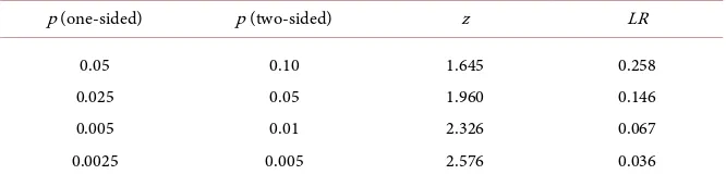
to LR leads to an evidential equivalence displayed in Table 2.

A likelihood ratio near 0.15 is the evidential equivalent of a two-sided p-value near 0.05. The 1 in 20 rule applied to the likelihood ratio

(

LR<0.05

)

would

translate to a more stringent rule than the p<0.05 rule prevalent throughout

much of statistical practice. Table 2 is our link between two seemingly disparate approaches to quantifying evidence.

We still need a way to unambiguously connect the p-value to the likelihood ratio for problems outside of the regular case. Evidence measured on the like-lihood ratio scale is interpreted the same, whether from the regular case or not. Thus, we have an unambiguous measure of evidence against a null hypothesis

:

o o

H θ θ= on the likelihood ratio scale. We can read this in Table 2 as the

right most column. The answer we are looking for can be found by reading Ta-ble 2 from right to left. For any likelihood ratio statistic, there exists a translated

z statistic. Note that such a z statistic need not actually exist. We are only

interested in the equivalence to some value on the evidence scale. We can then translate this z into a p-value measure of evidence. In other words, any

[image:6.595.207.540.649.735.2]

like-lihood ratio can be uniquely translated into a p-value. We thus have a p-value, or at least an evidential measure on the p-value scale, which satisfies the likelihood principle.

Table 2. LR scale of evidence.

p (one-sided) p (two-sided) z LR

0.05 0.025 0.005 0.0025

0.10 0.05 0.01 0.005

1.645 1.960 2.326 2.576

Let’s demonstrate the computation of a likelihood based p-value by returning one last time to the simple binomial example. The likelihood function is not of the regular case, but that does not matter. Earlier in this section, we computed

( )

_o 0.208.

LR θ = We can connect a likelihood ratio to a z statistic by solving

(1) as

( )

2 ln o .

z= − LR θ

For our problem, we get z=1.77. We can easily connect a z statistic to a

p-value. Since the alternative hypothesis is one-sided, we can compute

0.0384.

LRp= No matter the frequentist intention for the experiment, the

cal-culations for LRp remain the same. The result is an unambiguous p-value

cal-culation. One can use a p-value measure of evidence while adhering to the like-lihood principle.

Any testing problem where evidence can be quantified through the likelihood function can also be quantified through a uniquely defined measure on the p-value scale. We can think of this measure as defining a p-value which does in-deed satisfy the likelihood principle.

4. Bayes Factors

A second deficiency to be addressed is that the p-value as an assessment of evi-dence accounts only for the direction of the alternative hypothesis, and not for a specified alternative value. We will explore this issue further by studying the Bayes factor. Let’s demonstrate the use of Bayes factors for quantifying evidence through a development analogous to the regular case of the likelihood function. Consider a test statistic Z distributed conditional on parameter δ as

( )

,1 .

Z δ ∼N δ Under this parameterization, δ is interpreted as n times a

dimensionless measure of effect size. So, the mean of Z grows with the sample

size when the effect size is nonzero.

We are interested in testing the null hypothesis of no effect, H_o:δ =0.

Taking a Bayesian approach, define π_o =P

(

δ =0

)

as the prior probability on

the null. For now, we take a point prior on the alternative as well;

(

)

1 P 1 ,

π = δ δ= where πo+π1=1. The posterior probability on the null

con-ditional on observing Z =z becomes

(

)

_{( )}

( )

_{( )}

1 1

o o o

o o

f z

P H z

f z f z

π

π π

=

+

where fo,f1 are the null and alternative densities, respectively, for Z. The Bayes factor, BF, is introduced by writing the posterior odds as

(

)

(

)

01 1 1

o o

P H z

BF P H z

π π

= ⋅

quantify evidence by the change in probability from the prior (before data) to the posterior (after data). The Bayes factor measures this change as the ratio of the posterior odds to the prior odds. If BF01<1, the odds in favor of the null have decreased, so the data evidence is against the null hypothesis. If BF01>1, the odds in favor of the null have increased after data observation. The evidence from the data is then in favor of the null. (Bayes factors, unlike p-values and li-kelihood ratio statistics, can be used to determine when evidence favors a null hypothesis.)

Let’s consider a simple example to show why the specification of an alterna-tive hypothesis matters when defining a measure of evidence. Suppose we are testing H_o:δ =0 against the specific alternative H₁:δ =2. Suppose further

that we observe z=1.645. The one-sided p-value of p=0.05 represents

moderate evidence against the null according to the Fisher scale. The Bayes fac-tor is computed to be BF01=0.275. As BF01<1, the data evidence is against

the null, consistent with the information from the p-value. Now, consider testing

: 0

o

H δ = against the specific alternative H₁:δ =4. Recall that δ depends

on the sample size. We can imagine a test here similar to the first, but with a larger sample size. Suppose we again observe z=1.645. On the surface, it

would appear that we have replicated the result from the first experiment. Once again, there is evidence against the null as judged by the p-value. The Bayes fac-tor tells us a different sfac-tory. For the replicated data, we compute BF01=4.1. Since BF01>1, the data evidence is actually in favor of the null hypothesis. Neither hypothesis is particularly compatible with the observed data, but the null model provides a better fit than the specified alternative. A small p-value is only an indication of the null fit. To properly quantify evidence, one needs an assess-ment under the alternative hypothesis as well. This idea is summarized in [8]: “The clear message is that knowing the data are rare under Ho is of little use

unless one determines whether or not they are also rare under H1.”

Let’s make the problem more general by taking a continuous prior over the alternative values for δ. Write δ δ ≠ ∼0 π δ

( )

. The Bayes factor is now

writ-ten as

(

)

( )

2

01

2

1 exp

2

. 1

exp d

2 z BF

z δ π δ δ

₋ 

 

 

=

_{− −} 

 

 

∫

(2)

It is worth noting that π δ

( )

must be a proper prior in order for the integral in (2) to exist. A Bayesian cannot fall back upon objective or noninformative priors for testing problems involving a precise null hypothesis. That one must specify a proper alternative prior also follows intuitively from our discussion on how the Bayes factor as a measure of evidence requires a characterization of the alternative.

setting a specific alternative hypothesis. This idea is not new, nor is it without merit. Fisher did not consider the specification of an alternative to be an impor-tant aspect of a testing problem. The feud between Fisher and Neyman was in part over the Neyman-Pearson reliance on error rates [9]. One could argue, as Fisher did, that the goal of a testing problem should be to identify any evidence which contradicts a null hypothesis. Where does this leave us in our attempt to link these contrasting philosophies for quantifying evidence? While we will not find a complete success in this regard, it does happen that one can partially bridge the gap between p-values and Bayes factors.

As with p-values and likelihood ratio statistics, smaller values of Bayes factor

01

BF represent greater evidence against the null hypothesis. An evidence scale

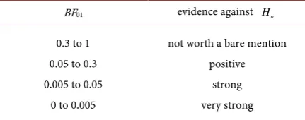
for interpreting a Bayes factor was initially proposed by Jeffreys, then modified slightly [10] (see Table 3).

Let’s continue with our discussion on the regular case. The Bayes factor in (2) requires specification of an alternative; a p-value does not. The p-value philoso-phy is consistent with the idea of searching for evidence across the entirety of the alternative space. This idea can be put into play by determining the specific al-ternative best supported by the observed data. In our problem, that idea trans-lates into an alternative prior placing full weight at δ1=z. The maximum de-nominator value of 1 is achieved for this use of a prior. The result is a lower bound for the Bayes factor, given by

2 01

1

exp .

2

BF ≥ _− z _

 

(3)

We further recognize the right hand side of the inequality in (3) as the like-lihood ratio statistic from our discussion in Section 3. In fact, one can show that the inequality BF01≥LR

( )

θo holds for the general problem of testing

: .

o o

H θ θ= We showed how to link the p-value, and z statistic, to the

like-lihood ratio statistic. We then extend this link to the (minimum) Bayes factor through inequality (3).

An extended discussion of the positive implications which may arise from a shift to thinking about p-values in conjunction with Bayes factors is provided in

[11]. We add to this discussion by noting how the relationship between a p-value and a Bayes factor puts the results from Section 3 in a different light. Let’s return to the coin spinning example. The p-value for testing the hypothesis of a fair coin was computed to be p=0.056. The corresponding likelihood ratio

[image:9.595.265.481.646.731.2]

statis-tic, LR

( )

θ =o 0.16, represents a lower bound on BF01. Since small values in-

Table 3. BF scale of evidence.

BF01 evidence against Ho

0.3 to 1 0.05 to 0.3 0.005 to 0.05

0 to 0.005

not worth a bare mention positive

dicate stronger evidence, the likelihood ratio serves as an upper bound on the strength of evidence against the null. A Bayes factor BF01=0.16 would

consti-tute positive evidence against the null on the Jeffreys scale, similar to a descrip-tion of moderate evidence as determined from the p-value on the Fisher scale. But since the actual Bayes factor BF01 cannot be reconstructed precisely, a

bound on the evidence measure is the best one can achieve from the p-value. An interpretation of a p-value as a measure of evidence must be tempered by the realization that such a measure is computed under the best case scenario for the alternative. This is a good reminder for an investigator to be careful about over-stating evidence summarized through a p-value.

5. Concluding Remarks

An understanding of what can be implied from hypothesis testing results is a necessary obligation for a conscientious scientist. There is much debate as to the role of the p-value in scientific reasoning and discussion. Criticism over the use of the p-value tends to focus on its deficiencies in comparison to more rigorous-ly defined evidential measures. We have seen, however, that a p-value measure of evidence can be defined under the likelihood principle. Furthermore, we have seen that the information from a p-value is related to a measure of evidence pro-vided by a Bayes factor. The connection between p-values and likelihood based measures of evidence broaden the use of the p-value in statistical hypothesis testing. Even if one desires a quantification of evidence through the likelihood principle, or through a Bayes factor, the p-value can still be a useful instrument.

References

[1] Wasserstein, R. and Lazar, N. (2016) The ASA’s Statement on p-Values: Context, Process, and Purpose. The American Statistician, 70, 129-133.

https://doi.org/10.1080/00031305.2016.1154108

[2] Efron, B. (2013) Large-Scale Inference: Empirical Bayes Methods for Estimation, Testing, and Prediction. Cambridge University Press, Cambridge.

[3] Gelman, A. and Robert, C. (2013) Revised Evidence for Statistical Standards.

Pro-ceedings of the National Academy of Sciences, 111, 19.

[4] Pawitan, Y. (2013) In All Likelihood: Statistical Modelling and Inference Using Li-kelihood. Oxford University Press, Oxford.

[5] Berger, J. and Wolpert, R. (1988) The Likelihood Principle: A Review, Generaliza-tions, and Statistical Implications. Institute of Mathematical Statistics, Hayward, CA.

[6] MacKenzie, D. (2002) Euro Coin Accused of Unfair Flipping. New Scientist.

http://www.newscientist.com/article/dn1748

[7] Agresti, A. (2013) Categorical Data Analysis. Wiley, Hoboken, NJ.

[8] Sellke, T., Bayarri, M. and Berger, J. (2001) Calibration of p-Values for Testing Pre-cise Null Hypotheses. The American Statistician, 55, 62-71.

https://doi.org/10.1198/000313001300339950

[10] Kass, R. and Raftery, A. (1995) Bayes Factors. Journal of the American Statistical

Association, 90, 773-795.https://doi.org/10.1080/01621459.1995.10476572

[11] Goodman, S. (2001) Of p-Values and Bayes: A Modest Proposal. Epidemiology, 12, 295-297.https://doi.org/10.1097/00001648-200105000-00006

Submit or recommend next manuscript to OALib Journal and we will pro-vide best service for you:

 Publication frequency: Monthly

 _{9 subject areas of science, technology and medicine}

 Fair and rigorous peer-review system

 Fast publication process

 _{Article promotion in various social networking sites (LinkedIn, Facebook, Twitter,}

etc.)

 _{Maximum dissemination of your research work}

Submit Your Paper Online: Click Here to Submit