Estimation Based on Progressive First-Failure
Censored Sampling with Binomial Removals
*
Ahmed A. Soliman1, Ahmed H. Abd Ellah2, Nasser A. Abou-Elheggag2, Rashad M. El-Sagheer3
1Faculty of Science, Islamic University, Madinah, Saudi Arabia 2Mathematics Department, Sohag University, Sohag, Egypt
3Mathematics Department, Faculty of Science, Al-Azhar University, Nasr-City, Cairo, Egypt Email: [email protected]
Received April 27, 2013; revised May 28, 2013; accepted June 15, 2013
Copyright © 2013 Ahmed A. Soliman et al. This is an open access article distributed under the Creative Commons Attribution Li-cense, which permits unrestricted use, distribution, and reproduction in any medium, provided the original work is properly cited.
ABSTRACT
In this paper, the inference for the Burr-X model under progressively first-failure censoring scheme is discussed. Based on this new censoring were the number of units removed at each failure time has a discrete binomial distribution. The maximum likelihood, Bootstrap and Bayes estimates for the Burr-X distribution are obtained. The Bayes estimators are obtained using both the symmetric and asymmetric loss functions. Approximate confidence interval and highest poste- rior density interval (HPDI) are discussed. A numerical example is provided to illustrate the proposed estimation meth- ods developed here. The maximum likelihood and the different Bayes estimates are compared via a Monte Carlo simu- lation study.
Keywords: Burr-X Distribution; Progressive First-Failure Censored; Bayesian and Non-Bayesian Estimations; Loss
Function; Bootstrap; Random Removals
1. Introduction
Censoring is common in life-distribution work because of time limits and other restrictions on data collection. Censoring occurs when exact lifetimes are known only for a portion of the individuals or units under study, while for the remainder of the lifetimes information on them is partial. However, when the lifetimes of products are very high, the experimental time of a type II censor- ing life test can be still too long. A generalization of type II censoring is progressive type II censoring, which is useful when the loss of live test units at points other than the termination point is unavoidable. Johnson [1] de- scribed a life test in which the experimenter might decide how to group the test units into several sets, each as an as- sembly of test units, and then run all the test units simul- taneously until occurrence of the first failure in each group. Such a censoring scheme is called first-failure censoring. Wu and Kuş [2] obtained maximum likelihood estimates, exact confidence intervals and exact confidence regions for the parameters of Weibull distribution under the pro- gressive first-failure censored sampling. Note that a first- failure censoring scheme is terminated when the first
failure in each set is observed. If an experimenter desires to remove some sets of test units before observing the first failures in these sets this life test plan is called a progressive first-failure censoring scheme which recently was introduced by Wu and Kuş [2]. Recently, the estima- tion of Parameters from different lifetime distribution bas- ed on progressive type II censored samples is studied by several authors including Gupta et al. [3], Childs and Ba- lakrishnan [4], Siu keung tse et al. [5], Mosa and Jaheen [6], Ng et al. [7], Wu and Chang [8], Balakrishnan et al. [9], Wu [10], Soliman [11], and Sarhan and Abuammoh [12]. But in some reliability experiments, the number of patients dropped out the experiment cannot be pre-fixed and it is random. In such situations, the progressive cen- soring schemes with random removals are needed. There- fore, the purpose of this paper is to develop a Bayes esti- mation (symmetric and asymmetric loss functions) for the parameters of Burr-X distribution under the progressive first-failure censoring plan with random removals and construct the bootstrap confidence interval for the para- meters.
If X follows a Burr-X distribution, then the probabi- lity density function (pdf) and cumulative distribution
*Mathematics Subject Classification: 6
function (cdf) of X are given respectively by
2 exp
2
1 exp
2
x x x
1, ,x 0,
, x,0.k
R
XR R
h
m th
f x
: : :
m m n k R
n m
k
(1)
1 exp
2F x x (2) The rest of this paper is organized as follows. In Sec- tion 2, we describe the formulation of a progressive first- failure censoring scheme as described by Wu and Kuş [2]. The point estimation of the parameters of Burr-X distri- bution and binomial distribution based on the progressive first-failure censoring scheme is investigated in Section 3. In Section 4, we discuss the approximate interval esti- mation and highest posterior density interval (HPDI) for the Burr-X distribution under the progressive first-failure censored sampling plan. A numerical examples are pre- sented in Section 5, for illustration. In Section 6 we pro- vide some simulation results in order to give an assess- ment of the performance of the estimation method.
2. A Progressive First-Failure Censoring
Scheme
In this section, first-failure censoring is combined with progressive censoring as in Wu and Kuş [2]. Suppose that n independent groups with items within each group are put in a life test, 1 groups and the group in which the first failure is observed are randomly removed from the test as soon as the first failure (say 1: : :m n k) has occurred, 2 groups and the group in which the second failure is observed are randomly removed from the test as soon as the second failure (say 2: : :m n k) has occurred, and finally m groups and the group in which the failure is observed are randomly removed from the test as soon as the failure (say
) has occurred. The
1: : :m n k 2: : :m n k m m n k: : : are called progressively
first-failure-censored order statistics with the progressive censoring scheme . It is clear that
1 2 m . If the failure times of the items originally in the test are from a continuous population with distribution function
XR
X
R R m
R n
R
m t
X
X X
R
n
R R
R
F x and prob- ability density function f x
, the joint probability den- sity function for 1: , 2: is given by
R R: :
m n k R
X XRm n k:: , , m
R : : :m n k
XR
:
1 1 : :
1 j ,
k k n k
R
: : :
0 xm m n kR ,
1,2, , 1: : : 2: : : : :
: : : :
1
, , ,
m m n k m n k m m n m
m
j m n k j m j
f x x x
ck f x F x
R R (3)
1: : :m n k 2: : :m n k
x x
R R (4)
where
1 2c n n R n R
n R R
1 1 2
1
1 1
1 .
m R
R m
(5)
There are four special cases:
The first one if R 0, ,0
(
3
)
1 k , Equation reduces to the joint probability density function of first-failure- censored order statistics. The second case if , Equation (3) becomes the joint probability density func- tion of the progressively type II censored statistics. The third case if k1 and R
0, ,0
, then nm which corresponds to the complete sample. The last one if k1 and R
0, , n m
, , ,
XR XR XR
1 1 k
, then type II censored order statistics are obtained.
Also it can be seen that 1: : :m n k i m n k: : : m m n k: : :
can be viewed as a progressively type II censored sample from a population with distribution function
F x
m n k
. For this reason, results for the progres- sively type II censored order statistics can be extended to progressively first-failure-censored order statistics easily.
Obviously, although more items are used (only of items are failures) in the progressive first-failure censoring plan than in others, it has advantages in terms of reducing test cost and test time.
3. Point Estimation
In many cases, there will be an obvious or natural candi- date for a point estimator of a particular parameter. For example, the sample mean is a natural candidate for a point estimator of the population mean. In this section, we estimate and , by considering maximum likeli- hood, bootstrap and Bayes estimates. In Bayesian tech- nique, we consider both symmetric (Squares Error, SE) loss function and asymmetric (Linear Exponential, LINEX and General Entropy, GE) loss functions.
p
xR 1, 2, ,
i m
3.1. Maximum Likelihood Estimation (MLE) Let i m n k: : : ,
R
, be the progressively first-fail- ure censored order statistics from a Burr-X distribution, with censoring scheme from (3), the likelihood func- tion is given by
1
1
1 1 1 1
0 0 1
;
exp 1 ln ,
m
m
k R
k R m
m m
i i
J J i
L x
ck T x G j U
(6) where
2
1
2
1
2 exp , 1 exp ,
m
i i i i i
i
T x x x U U x
(7)
1 1
1
1 1 1 1
1 j jm m ,
m
k R k R
G
j j
c
(8)
where is defined in (5) and xi is used instead of
: : :m n k. Now, suppose that any group
xR
i being re-
with the same probability . Then, the number of groups removed at each failure time follows a binomial distribu-
p 1 1 i l l
n m r p m
1
n m r1,p
, , 1.
i m
tion with parameters and where is predetermined before the testing. Therefore
11 1 1 r n m r p r P R 2,3 (9) and for
11
1 1
1 n m il rl,
r R r R r
n m r
p p r
1 i2,3, , 1
i m 1 1 1 1 , , i
i i i i i r l l i P R r n (10)
where 0 i m
l1rl,
1 1 2 2 1 1 3 3
1 1 2 2, , 1 1
,2 2, 1 1
m m
P R R r R r P R r R r R r
P R R r R r
m m
r P
r P Rr
(11) hence
1 1 1 11 11
1 1
!
! !
1 mi i.
i
m m
i i i
i
m n m m i r r
n m r
r n m r
p p
R i m i P R (12)Suppose further that i is independent of x . Then the likelihood function takes the following form
, ;x R,
L
;x Rr P R
r
,L p (13)
1 1 1 1 1 1 1 1 1 10 0 1
1
, ; ,
exp 1 ln
1 m m m m i i i i
k R m
i i
j j i
m n m m i r r
L p x
c T x G j U
p p
k R m r (14) Using (6), (12) and (13) we can write the likelihood function as
,
1 ; 2
,L , ;p x r c T x L x L Rr (15)
where
1 1 m m i ck n c r n
1 1 !! m !
i i i
m
m r
and
1 1
1 1 1 1
1
0 0
; e
1
xp 1 ln
m
m
k R
k R m
m
i i
j j i
L x G j U
. (16) and
1
1
1 mim m i r i .
1 L p 1 1 1 2 m i
i r m n
L Rr p p (17) It is obvious that in Equation (16) does not in-
volve . Thus the maximum likelihood estimate (MLE) of can be derived by maximizing Equation (16) di- rectly. On the other hand, in Equation (17) does not depend on the parameter 2
L ,
then the MLE of can be obtained directly by maximizing Equation (17). In particular, after taking the logarithms of
p
L1 and
2 , the MLE’s of
L p and can be found by sol- ving the following equations
p
1
1
1 1 1 1
1
0 0 1
log
1 ln 0
m
m
k R
k R m
i i
j j i
L m
G j U
(18)
2 1 1 1 1 log 1 1 0. 1 m m i i i i L p pm n m m i r
r p p
1
1
1 1 1
1 1
0 0 1
ˆ m 1 ln ,
m
k R
k R m
ML i i
j j i
m G j U
(19)
Thus we find
(20) and 1 1 1 1 ˆ 1 1 m i i ML m i i r pm n m m i r
. (21)3.2. Bootstrap Confidence Intervals
In this subsection, we use the parametric bootstrap per- centile method suggested by Efron [13] to construct con- fidence intervals for the parameters. The following steps are followed to obtain a progressive first-failure censor- ing bootstrap sample from Burr-X distribution with pa- rameter and binomial distribution with parameter based on simulated progressively first-failure censored data with random removals set.
p
From the original data 1: : :m n k 2: : :m n k , m m n kR: : :
and 1,R2, ,Rm
, ,
xxR xR x
RR compute the ML estimates of the parameters and p by Equations (20) and (21).
Use and p to generate a bootstrap sample x and R with the same values of
, ; 1
R m i
1 1 , 2, ,
i m using algorithm presented in
Balakrishnan and Sandhu [14] with distribution func- tion F x
k see Wu and Kuş [2].
As in Step 1, based on x compute the bootstrap sample estimates of and p, say and p.
Repeat steps 2-3 N times representing N boot- strap MLE’s of
,p
based on N different boot- strap samples. Arrange all s and p s , in an ascending order to obtain the bootstrap sample , N
l
1, 2,
,l l
1, 2
l (where 1 ,2 p). Let G z
P
l
.
z
be the cumulative distribution function of 1 Define for given z. The approximate bootstrap
1 lboot G z
100 1 % confidence interval of l is given by
1
, .
2 lboot 2
u u lboot (22)
3.3. Bayes Estimation
The Bayesian inference procedures have been developed under the usual SE loss function (quadratic loss), which is symmetrical, and associates equal importance to the losses due to overestimation and underestimation of equal magnitude. However, such a restriction may be imprac- tical. For example, in the estimation of reliability and failure rate functions, an overestimation is usually much more serious than an underestimation; in this case the use of asymmetrical loss function might be inappropriate, as has been recognized by Basu and Ebrahimi [15], and Can- field [16].
A useful asymmetric loss known as the LINEX loss function, was introduced by Zimmer et al. [17], and was widely used in several papers by Balasooriya and Bala- krishnan [18], Soliman [19] and Soliman [20]. This func- tion rises approximately exponentially on one side of ze- ro, and approximately linearly on the other side. Under the assumption that the minimal loss occurs at , the LINEX loss function for uu
,
can be expressedas
1
u u
, u
ea
L a 1, a0, (23) where is an estimate of u.
The sign, and magnitude of a
0
a
0
a represent the direc- tion, and degree of symmetry. ( means overestima- tion is more serious than underestimation, and
means the opposite). For
a closed to zero, the LINEX loss function is approximately the Squared Error (SE) loss, and therefore almost symmetricThe posterior-expectation of the LINEX loss function of (23) is
1.u u
u
a u E u
exp a u
exp u
E L u u
E a
(24)
where u is equivalent to the posterior-expectation with respect to the posterior . The Bayes esti- mator
E
pdf u BL
u of u under the LINEX loss function is the value u, which minimizes (24)
log u exp ,
uBL 1 E au
a
(25)
provided that
au
exists, and is finite.
exp u E
Another useful asymmetric loss function is General Entropy (GE) loss
2 , log 1
b
u u
L u u b
u u
.
uu
(26)
whose minimum occurs at . This loss function is a generalization of the Entropy-loss used in several papers where b1 by Dey et al. [21], Dey and Liu [22]. When
, a positive error 0
b
uu
causes more serious consequences than a negative error. The Bayes estimateBL
u of u under GE loss (26) is
1bb BG u
u E u (27) b
E u provided that u
Now, we assume that the parameters exists, and is finite.
and be-have as independent random variables, and we use gam- ma prior distribution with known parameters
p
,
for .
The prior pdf of takes the form
1
1 exp , 0, , 0,
p , .
(28)
while has Beta prior distribution with known para- meters
That is
1
12
1
1 , 0 1, , 0. ,
p p p p
B
(29) is
Therefore the posterior (pdf) of
1 1
1
1 1
0 ;
,
; d
L x
x
L x
(30)
where L1 ;x
the likelihood function and 1
the prior density function. Applying (16) and (28), the mar- ginal posterior (pdf) of given by
1
1
1
1
1 1 1 1
1
0 0
1 1 1 1 1
0 0
exp ,
m
m
m
m
k R k R
m
j j j
k R k R
m j j j
G q
x
m Gq
1
1 ln ,
m
j i i
i
q j U
(31)
where
(32)
We notes that the posterior distribution of is Gam- ma with parameters
m
and qjp
Similarly, the po- sterior (pdf) of is
2 2
2 1
2 2
0
, ,
d
L R r p
p x r
L R r p p
(33)
2
where L Rr the likelihood function and 2 p
p
the prior density function.
1
21 ,
p x r p
B 1
, 1 p ,
1
1 m i.
i
m i r
p (34) where
1 1 , m i l rm n m
(35)We notes that the posterior distribution of is Beta with parameters and
.
3.3.1. Symmetric Bayes Estimation
SE loss function: Under SE loss function, the estimator
of a parameter (or given function of the parameters) is its posterior mean. Thus, Bayes estimators of the parameters are obtained by using the posterior densities (31) and (34). The Bayes estimators BS
and pBS
of the para- meters and are p
0 1
x dBS E x
(36) from (31) resulting in
1 1 1 1 1 1 1 1 0 0 1 1 1 1 0 0 m m m m k R k R j j BS k R k Rj j Gq
1 , m j m jm Gq
G
(37)
where and qj are defined in (8) and (32). Similar- ly,
p 2
p x r, d ,
p
1 0 BS p
p E p x
(38) from (34) resulting in
, BS p
(39)
where and are defined in (35).
3.3.2. Asymmetric Bayes Estimation
LINEX loss function: If in (25), u, then the Bayes estimator BL
, of the parameter relative to LINEX loss function is
a
1
x d ,0 1 log exp BL a
(40) and from (31), we get
1 1 1 1 1 1 1 1 0 0 1 1 1 1 0 0 1log m m m m k R k R m j j jBL k R k R
m j
j j
G a q
a Gq
up
. (41)
Similarly, if in (25), , then the Bayes estimator BL
p , of the parameter relative to LINEX loss func- tion is p
1 2 0 1log exp d ,
BL
p ap p x p
a
(42)
and from (34), we obtain
01
1
11 1
log exp 1 d .
, BL
p
ap p p p
a B
(43) One can use a numerical integration technique to get the integration in (43).General Entropy loss function: Let u, in (27), then the Bayes estimate BG
, of parameter relative to the General Entropy loss function is
1 1 0 d , b b BG x
(44)and from (31), we obtain
1 1 1 1 1 1 1 1 1 0 0 1 1 1 1 0 0 . m m m m b k R k R m b j j j
BG k R k R
m j
j j
m b Gq
m Gq
u p (45) Put in (27), then the Bayes estimator pBG of the parameter relative to General Entropy loss func- tion is
p
1 1 2
0 d ,
b b
BG
p p p x p
(46) from (34), resulting in
1
. b BG b p b , (47)
4. Interval Estimation
4.1. Approximate Interval Estimation
The asymptotic variances and covariances of the MLE for parameters and are given by elements of the inverse of the Fisher information matrix
p
2
; , 1, 2. ij
L
E i j
p
I (48)
1
2 2
2
2 2
2 ,
var
p
L L
p
L L
0 , 0 var p
p p
(49)
with
2
2 2,
L m
(50)
1 1
1 1
2 1
m m
i i
i i
r m n m m i r
L
p p p
2
2 2
1
. (51)
The asymptotic normality of the MLE can be used to compute the approximate confidence intervals for pa- rameters and p. Therefore,
1
100% confi- dence intervals for parameters and p become
2 var and 2 var ,
Z p Z p
(52) where Z2 is the percentile of the standard normal dis- tribution with right-tail probability 2.
4.2. Highest Posterior Density Interval (HPDI) In general, the Bayesian interval estimation is much more direct than frquentest classical method. Now, having ob- tained the posterior distribution p
Data
we ask, “How likely is it that the parameter lies within the specified interval
L, U
?” Bayesian call this intervalbased on the posterior distribution a “credible interval”. The interval
L, U
is said to be a
1
100%credible interval for if
ata
d 1 .U
L
p D
(53)For the shortest credible interval, we have to minimize the interval
L, U
subject to the condition (53)which requires
L
U
.P Data P Data (54) As interval
L, U
which simultaneously satisfies (53) and (54) is called the “shortest” 1
100% cre- dible interval. A highest posterior density interval (HPDI) is such that the posterior density for every point inside the interval is greater than that for every point outside of it. For a unimodal, but not necessarily symmetrical pos- terior density, the shortest credible and the HPD intervals are identical. We now proceed to obtain the
1
HPD intervals for the parameters
100% and
Consider the posterior distribution of
. p in (31). The
1
100% HPDI
L, U
for the parameter isgiven by the simultaneous solution of the equations
1 , 1 and 1 , 1 , .
U
L
L U
x r x r x r
p
(55) Similarly, using the posterior pdf of in (34), the
1
100% HPDI pL,pU for the parameter is p given by the simultaneous solution of the equations
2 , 1 and 2 , 2 , .
U
L
p
L U
p
p x r p x r p x r
0.79
(56) To obtain the HPDI from (55) and (56), one may em- ploy any mathematical package such as Mathematica, to get the intervals.
5. Numerical Example
Example 1: (simulated data) To illustrate the use of the
estimation methods proposed in this paper. A set of data consisting of 75 observations were generated from a Burr-X distribution with parameter , and ran- domly grouped into 15 sets. The generated data are listed below:
0.3194 0.4661 0.8348 0.1150 0.1230 0.2136 0.1373 0.2053
0.7253 0.7738 0.9407 0.1516 0.5111 0.4148 0.1599 0.3227
0.9233 0.8316 0.9615 0.2006 0.9758 0.6618 0.4116 0.9088
0.9787 0.8461 0.9795 0.7353 1.2692 0.8632 0.4503 1.1337
0.9956 0.9732 1.2067 1.0935 1.8144 0.9698 1.0344 2.0543
0.1775 0.3165 0.2732 0.2832 0.2752 0.2814 0.2761
0.3363 0.7871 0.4714 0.6613 0.5764 0.7273 0.5616
0.5353 0.8052 0.5134 0.6790 0.7441 0.7602 0.6529
0.8312 0.8695 0.9356 0.9049 0.9939 1.2178 0.9328
1.9019 1.0115 1.1291 1.5136 1.2023 1.7956 1.2521
Now, we consider the following cases:
Case I: Progressive first-failure censored data with binomial removals.
Algorithm 1.
1) Specify the value of n. m 2) Specify the value of
3) Generate the value of the parameters and using the prior densities (28) and (29), for some given values of the prior parameters
p
, ,
and . 4) Generate a random number r1 from
,
.bio n m p
i r 1
1 , , i
i l
bio n m r p
, i2,3, , m1. mr
5) Generate a random numbers from
for each i
1 1
1 1
0 w
i i
l l
l l
m r
1 1 F x k
if 0 o. m
n m r n
r
Based on the above data, a progressive first-failure censored data with binomial removals were generated using the algorithm described in Balakrishnan and Sandhu [14] with distribution function
see Wu and Kuş [2].
The generated progressive first-failure censored data with binomial removals are: (0.115, 0.123, 0.1373, 0.1757, 0.2053, 0.2732, 0.2752, 0.2761, 0.2832, 0.4661), and R = (0, 3, 1, 0, 1, 0, 0, 0, 0, 0) Using the results pre- sented in previous sections, the different point estimates of and are computed. We denote to the MLEs, estimates using the bootstrap, Bayes estimate relative to SE loss, Bayes estimate relative to LINEX loss, and Bayes estimate relative to GE loss, respectively by
p
.ML, . Boot., .
BS, . BL and
. BG.15 5 k5
The results are dis- played in Table 1.
Case II: First-failure censoring data with n
(n ,m 1 and ).
The set of the first-failure censored data are: (0.115, 0.123, 0.1373, 0.1757, 0.2053, 0.2136, 0.2732, 0.2752, 0.2761, 0.2814, 0.2832, 0.3165, 0.3194, 0.4661, 0.8348). Different point estimates of are computed and the results are listed in Table 1.
Case III: Progressive type II censoring data with binomial removals.
A progressive type II censoring data with binomial
removals have been generated from complete sample using the algorithm described in Balakrishnan and
Sandhu [14], with ( and
). i.e. 50 failure times are ob- served and 25 failure times are censored using censored scheme . The generated data are:
(0.115, 0.123, 0.1516, 0.1599, 0.2006, 0.2053, 0.2136, 0.2752, 0.2761, 0.2814, 0.2832, 0.3165, 0.3194, 0.3227, 0.3363, 0.4116, 0.4148, 0.5111, 0.5134, 0.5616, 0.5764, 0.6529, 0.679, 0.7273, 0.7353, 0.7441, 0.7602, 0.7871, 0.8052, 0.8312, 0.8461, 0.8632, 0.8695, 0.9049, 0.9088, 0.9328, 0.9407, 0.9698, 0.9732, 0.9787, 0.9939, 0.9956, 1.0344, 1.0935, 1.1291, 1.2067, 1.2178, 1.5136, 1.7956, 1.8144 ). The results of different Bayes estimates of
75, 50,
n m k
, 2,3,1,0,0, 2,042
R
1,p 0.4
9,8 R
and p are also, listed in Table 1.
Case IV: The complete sample data with
(n m 75 and k1)
The results of point estimates of the parameter and are shown in Table 1.
p
[image:7.595.95.251.86.127.2]Based on different type of censoring described above, the 95% credible intervals of
Table 1. Different point estimates of and for all cases with
p
,p
0.79,0.4
. .BL .BG
Cases (.) .ML .Boot. .BS a 2 a2 b 2 b2
0.7724 0.7863 0.7697 0.7823 0.7578 0.7776 0.7463
I p
0.3571 0.3974 0.3529 0.3659 0.3405 0.3705 0.2887
II 0.7818 0.7936 0.7775 0.7885 0.7670 0.7844 0.7570 0.7656 0.7723 0.7608 0.7701 0.7518 0.7667 0.7428
III p
0.3906 0.3985 0.3881 0.3916 0.3846 0.3925 0.3740
IV 0.7802 0.7902 0.7745 0.7825 0.7667 0.7796 0.7592
Table 2. 95% confidence intervals for and under progressive first-failure censored samples when
p
,p
0.79,0.4
.ACI Boot CI HPDI
Cases (.)
[L,U] [L,U] [L,U]
[0.5524, 0.9925] [0.6965, 0.8056] [0.5737, 1.0069]
I p
[0.1061, 0.6081] [0.1905, 0.5000] [0.1520, 0.5866]
II [0.3862, 1.1775] [0.5285, 0.6365] [0.5911, 0.9964]
[0.5753, 0.9559] [0.7015, 0.8076] [0.5864, 0.9606]
III p
[0.2711, 0.5102] [0.3906, 0.4902] [0.2758, 0.5066]
IV [0.6036, 0.9568] [0.6928, 0.8798] [0.6102, 0.9581]
6. Simulation Study
In order to compare the different estimators of the pa- rameters, we simulated
1000
progressively first-fail- ure-censored samples from a Burr type X distribution with the values of parameters , and different combinations of , and censoring random schemes The samples were simulated by using the algorithm described in Balakrishnan and Sandhu [14]. A simulation was conducted in order to study the properties and compare the performance of the Bayes estimator with maximum likelihood estimator.
,p
0.79,0.4
, ,
n m k
.
R
R
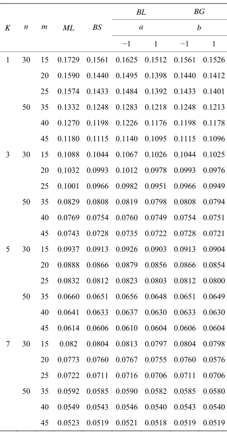
The mean square error (MSE) of the Bayes estimations and maximum likelihood estimations are computed over different combination of the censored random scheme as shown in Tables 3 and 4. To asses the effect of
the shape parameters a and b from Tables 3 and 4, one
can see that the asymmetric Bayes estimates (BL, BG) of the (MSE) of the parameters and are overestimates for (
p 0,
a and are obtained
using approximate confidence interval (ACI), confidence interval based on bootstrap re-sampling method (Boot CI), and the highest posterior density interval (HPDI). All the results are listed in Table 2.
p
b0), and when ( ) the (MSE) of the parameters are underestimates. Also, the MSE of Bayes estimates are smaller than MSE of the MLE, when
0, a b0
Table 3. Mean square errors of the parameter .
BL BG
a b
K n m ML BS
−1 1 −1 1
1 30 15 0.1729 0.1561 0.1625 0.1512 0.1561 0.1526
20 0.1590 0.1440 0.1495 0.1398 0.1440 0.1412
25 0.1574 0.1433 0.1484 0.1392 0.1433 0.1401
50 35 0.1332 0.1248 0.1283 0.1218 0.1248 0.1213
40 0.1270 0.1198 0.1226 0.1176 0.1198 0.1178
45 0.1180 0.1115 0.1140 0.1095 0.1115 0.1096
3 30 15 0.1088 0.1044 0.1067 0.1026 0.1044 0.1025
20 0.1032 0.0993 0.1012 0.0978 0.0993 0.0976
25 0.1001 0.0966 0.0982 0.0951 0.0966 0.0949
50 35 0.0829 0.0808 0.0819 0.0798 0.0808 0.0794
40 0.0769 0.0754 0.0760 0.0749 0.0754 0.0751
45 0.0743 0.0728 0.0735 0.0722 0.0728 0.0721
5 30 15 0.0937 0.0913 0.0926 0.0903 0.0913 0.0904
20 0.0888 0.0866 0.0879 0.0856 0.0866 0.0854
25 0.0832 0.0812 0.0823 0.0803 0.0812 0.0800
50 35 0.0660 0.0651 0.0656 0.0648 0.0651 0.0649
40 0.0641 0.0633 0.0637 0.0630 0.0633 0.0630
45 0.0614 0.0606 0.0610 0.0604 0.0606 0.0604
7 30 15 0.082 0.0804 0.0813 0.0797 0.0804 0.0798
20 0.0773 0.0760 0.0767 0.0755 0.0760 0.0576
25 0.0722 0.0711 0.0716 0.0706 0.0711 0.0706
50 35 0.0592 0.0585 0.0590 0.0582 0.0585 0.0580
40 0.0549 0.0543 0.0546 0.0540 0.0543 0.0540
45 0.0523 0.0519 0.0521 0.0518 0.0519 0.0519
relative to both LINEX loss, and GE loss (for close to 0, and ) are the same as the SE loss Bayes es- timates. This one of the useful properties of working with the LINEX loss function we found that for different choices of k, , and censoring random scheme the MSE of the Bayes estimates based on symmetric and asymmetric loss functions perform better than MSE of the MLEs. when the effective sample proportion
a 1
b
n m
R
m n
increases, the MSE of each the Bayes estimation and maximum likelihood estimations reduce. Also the cen- soring scheme R n m , ,0
is most efficient Forall choices, it seems to usually provide the smallest MSE for each estimates of and p.
p
7. Conclusion
The purpose of this paper is to develop a Bayesian analy-
Table 4. Mean square errors of the parameter .
BG
BL
a b
n m BS
K ML
−1 1 −1 1
1 30 15 0.0865 0.0767 0.0779 0.0757 0.0767 0.0753
20 0.1056 0.0886 0.0901 0.0873 0.0886 0.0882
25 0.1518 0.1066 0.1098 0.1038 0.1066 0.1065
50 35 0.0871 0.0772 0.0783 0.0763 0.0772 0.0761
40 0.1065 0.0887 0.0904 0.0872 0.0887 0.0871
45 0.1618 0.1112 0.1148 0.1080 0.1112 0.1089
3 30 15 0.0856 0.0765 0.0774 0.0757 0.0765 0.0762
20 0.1052 0.0883 0.0899 0.0868 0.0883 0.0873
25 0.1498 0.1047 0.1081 0.1016 0.1047 0.1033
50 35 0.0835 0.0744 0.0754 0.0734 0.0744 0.0734
40 0.1037 0.0874 0.0889 0.0859 0.0874 0.0864
45 0.1464 0.1039 0.1068 0.1014 0.1039 0.1053
5 30 15 0.0879 0.0779 0.0790 0.0769 0.0779 0.0765
20 0.1065 0.0894 0.0910 0.0880 0.0894 0.0883
25 0.1512 0.1066 0.1098 0.1037 0.1066 0.1062
50 35 0.0857 0.0766 0.0776 0.0757 0.0766 0.0758
40 0.1095 0.0915 0.0932 0.0900 0.0915 0.0901
45 0.1471 0.1031 0.1063 0.1004 0.1031 0.1036
7 30 15 0.0879 0.0780 0.0791 0.0771 0.0780 0.0770
20 0.1070 0.0896 0.0912 0.0881 0.0896 0.0883
25 0.1564 0.1097 0.1129 0.1068 0.1097 0.1092
50 35 0.0861 0.0766 0.0776 0.0756 0.0766 0.0753
40 0.1065 0.0890 0.0907 0.0874 0.0890 0.0872
45 0.1546 0.1082 0.1115 0.1052 0.1082 0.1074
sis for Burr-X distribution under the progressively first- fialure censored sampling plan with binomial random re- movals. We studied point and interval estimations of pa- rameter of the Burr type X distribution. We derived the MLEs, Bayes estimators (BS, BL, BG). A simulation stu- dy was conducted to examine the performance of the MLE and the Bayes estimators.
8. Acknowledgements
The authors would like to express their thanks to the edi- tor, assistant editor and referees for their useful comments and suggestions on the original version of this manuscript.
REFERENCES
[image:8.595.309.535.100.526.2]search,” Elsevier, Amsterdam, 1964.
[2] S.-J. Wu and C. Kus, “On Estimation Based on Progres-sive First-Failure-Censored Sampling,” Computational Statistics and Data Analysis, Vol. 53, No. 10, 2009, pp. 3659-3670. doi:10.1016/j.csda.2009.03.010
[3] P. L. Gupta, S. Gupta and Ya. Lvin, “Analysis of Failure Time Data by Burr Distribution,” Communication Statis- tics Theory & Methods, Vol. 25, No. 9, 1996, pp. 2013- 2024. doi:10.1080/03610929608831817
[4] A. Childs and N. Balakrishnan, “Conditional Inference Procedures for the Laplace Distribution When the Ob- served Samples Are Progressively Censored,” Metrika, Vol. 52, No. 3, 2000, pp. 253-265.
doi:10.1007/s001840000092
[5] S. K. Tse, C. Y. Yang and H.-K. Yuen, “Statistical Ana- lysis of Weibull Distribution Lifetime Data under Type II Progressive Censoring with Binomial Removals,” Jour- nal of Applied Statistics, Vol. 27, No. 8, 2000, pp. 1033- 1043. doi:10.1080/02664760050173355
[6] M. A. M. Ali Mousa and Z. F. Jaheen, “Statistical Infer-ence for the Burr Model Based on Progressively Censored Data,” An International Computers & Mathematics with Applications, Vol. 43, No. 10-11, 2002, pp. 1441-1449.
doi:10.1016/S0898-1221(02)00110-4
[7] K. Ng, P. S. Chan and N. Balakrishnan, “Estimation of Pa- rameters from Progressively Censored Data Using an Al- gorithm,” Computational Statistics and Data Analysis, Vol. 39, No. 4, 2002, pp. 371-386.
doi:10.1016/S0167-9473(01)00091-3
[8] S.-J. Wu and C.-T. Chang, “Parameter Estimation Based on Exponential Progressive Type II Censored Data with Binomial Removals,” Information and Mangement Statis- tics, Vol. 13, No. 3, 2002, pp. 37-46.
[9] N. Balakrishnan, N. Knnan, C. T. Lin and H. Ng, “Point and Interval Estimation for Gaussian Distribution Based on Progressively Type-II Censored Samples,” IEEE Tran- sactions on Reliability, Vol. 52, No. 3, 2003, pp. 90-95.
doi:10.1109/TR.2002.805786
[10] S.-J. Wu, “Estimation for the Two-Parameter Pareto Dis- tribution under Progressive Censoring with Uniform Re- movals,” Journal of Statistical Computation and Simula- tion, Vol. 73, No. 2, 2003, pp. 125-134.
doi:10.1080/00949650215732
[11] A. A. Soliman, “Estimation of Parameters of Life from Progressively Censored Data Using Burr-XII Model,” IEEE Transactions on Reliability, Vol. 54, No. 1, 2005,
pp. 34-42. doi:10.1109/TR.2004.842528
[12] A. M. Sarhan and A. Abuammoh, “Statistical Inference Using Progressively Type-II Censored Data with Random Scheme,” International Mathematical Forum, Vol. 35, No. 3, 2008, pp. 1713-1725.
[13] B. Efron, “The Bootstrap and Other Resampling Plans,” CBMS-NSF Regional Conference Seriesin Applied Mathe- matics, Vol. 38, SIAM, Philadelphia, 1982.
[14] N. Balakrishnan and R. Asandhu, “A Simple Simulation Algorithm for Generating Progressively Type-II Censored Samples,” The American Statistican, Vol. 49, No. 2, 1995, pp. 229-230.
[15] A. P. Basu and N. Ebrahimi, “Bayesian Approach to Life Testing and Reliability Estimation Using Asymmetric Loss Function,” Journal of Statistical Planning and In- ference, Vol. 29, No. 1-2, 1991, pp. 21-31.
doi:10.1016/0378-3758(92)90118-C
[16] R. V. Caneld, “A Bayesian Approach to Reliability Esti- mation Using a Loss Function,” IEEE Transactions on Reliability, Vol. 19, No. 1, 1970, pp. 13-16.
[17] W. J. Zimmer, J. Bert Keats and F. K. Wang, “The Burr XII Distribution in Reliability Analysis,” Journal of Qua- lity & Technology, Vol. 30, No. 4, 1998, pp. 386-394. [18] U. Balasooriya and N. Balakrishnan, “Reliability Sampl-
ing Plans for Log-Normal Distribution Based on Progres- sively Censored Samples,” IEEE Transactions on Relia- bility, Vol. 49, No. 2, 2000, pp. 199-203.
doi:10.1109/24.877338
[19] A. A. Soliman, “Comparison of LINEX and Quadratic Bayes Estimators for the Rayleigh Distribution,” Communica- tions in Statistics Theory and Methods, Vol. 29, No. 1, 2000, pp. 95-107. doi:10.1080/03610920008832471 [20] A. A. Soliman, “Estimation of Parameters of Life from Pro-
gressively Censored Data Using Burr-XII Model,” IEEE Transactions on Reliability, Vol. 54, No. 1, 2005, pp. 34- 42.
[21] D. K. Dey, M. Ghosh and C. Srinivasan, “Simultaneous Estimation of Parameters under Entropy Loss,” Journal of Statistical Planning and Inference, Vol. 15, No. 2, 1987, pp. 347-363.
[22] D. K. Dey and P. L. Liu, “On Comparison of Estimation in Generalized Life Model,” Microelectron & Reliability, Vol. 32, No. 1-2, 1992, pp. 207-221.