www.hydrol-earth-syst-sci.net/19/1919/2015/ doi:10.5194/hess-19-1919-2015
© Author(s) 2015. CC Attribution 3.0 License.
Hydrological recurrence as a measure for large river basin
classification and process understanding
R. Fernandez1,2and T. Sayama1,3
1International Centre for Water Hazard and Risk Management, Public Works Research Institute, Tsukuba, Ibaraki, Japan 2National Graduate Institute for Policy Studies, Tokyo, Japan
3Now at Disaster Prevention Research Institute, Kyoto University, Kyoto, Japan
Correspondence to: R. Fernandez ([email protected])
Received: 30 May 2014 – Published in Hydrol. Earth Syst. Sci. Discuss.: 18 July 2014 Revised: 23 December 2014 – Accepted: 18 March 2015 – Published: 22 April 2015
Abstract. Hydrological functions of river basins are sum-marized as collection, storage and discharge, which can be characterized by the dynamics of hydrological variables in-cluding precipitation, evaporation, storage and runoff. The temporal patterns of each variable can be indicators of the functionality of a basin. In this paper we introduce a mea-sure to quantify the degree of similarity in intra-annual vari-ations at monthly scale at different years for the four main variables. We introduce this measure under the term of recur-rence and define it as the degree to which a monthly hydro-logical variable returns to the same state in subsequent years. The degree of recurrence in runoff is important not only for the management of water resources but also for the under-standing of hydrologic processes, especially in terms of how the other three variables determine the recurrence in runoff. The main objective of this paper is to propose a simple hy-drologic classification framework applicable to large basins at global scale based on the combinations of recurrence in the four variables using a monthly scale time series. We evaluate it with lagged autocorrelation (AC), fast Fourier transforms (FFT) and Colwell’s indices of variables obtained from the EU-WATCH data set, which is composed of eight global hy-drologic model (GHM) and land surface model (LSM) out-puts. By setting a threshold to define high or low recurrence in the four variables, we classify each river basin into 16 pos-sible classes.
The overview of recurrence patterns at global scale sug-gested that precipitation is recurrent mainly in the humid tropics, Asian monsoon area and part of higher latitudes with an oceanic influence. Recurrence in evaporation was mainly dependent on the seasonality of energy availability, typically
high in the tropics, temperate and sub-arctic regions. Recur-rence in storage at higher latitudes depends on energy/water balances and snow, while that in runoff is mostly affected by the different combinations of these three variables. Ac-cording to the river basin classification, 10 out of the 16 pos-sible classes were present in the 35 largest river basins in the world. In the humid tropic region, the basins belong to a class with high recurrence in all the variables, while in the subtropical region many of the river basins have low recur-rence. In the temperate region, the energy limited or water limited in summer characterizes the recurrence in storage, but runoff exhibits generally low recurrence due to the low recurrence in precipitation. In the sub-arctic and arctic re-gions, the amount of snow also influences the classes; more snow yields higher recurrence in storage and runoff. Our pro-posed framework follows a simple methodology that can aid in grouping river basins with similar characteristics of wa-ter, energy and storage cycles. The framework is applicable at different scales with different data sets to provide useful insights into the understanding of hydrologic regimes based on the classification.
1 Introduction
Vari-ations at seasonal scale are the most recognized patterns in most hydrological processes playing important roles in wa-ter resource management. Other climatological changes and additional anthropogenic pressure also add to the complexity of the hydrological cycle.
Regardless the complexity, the primary function of a river basin in the hydrological cycle is simply characterized with three main functions: collection, storage and discharge (Black, 1997). The collection function describes the different paths that supplied water from precipitation follows until it reaches a storage component. This collected water is stored at different states and locations within a basin. Water stor-age, as the first-order state variable of river basins, represents its hydrologic condition and serves as the link between col-lection and discharge regulating the timing and amount of collected water to be released. The discharge function refers to the processes that release the stored water in the form of evaporation back into the atmosphere or as runoff. Among these functions, the prediction and understanding of the re-lease as runoff has been of high importance to understand water hazards and resource management. Nevertheless, as runoff is highly dependent on the other two functions, un-derstanding the dynamics of water collection and storage is unavoidable in order to understand hydrological processes at river basins.
The importance of storage dynamics has been highlighted with emerging new concepts in watershed hydrology. Fill and spill (Spence and Woo, 2003; Tromp van Meerveld and McDonnell, 2006; Shaw et al., 2012), connectivity (McG-lynn et al., 2013) and threshold (Fu et al., 2013; Ali et al., 2013) are a few examples amongst various concepts of runoff generation mechanisms highlighting the importance of water storage and its capacity. Recent studies have demonstrated similar concepts at multiple scales based on water balance analysis (Sayama et al., 2011), combinations of soil mois-ture and streamflow measurements (Sidle et al., 2000) and numerical simulations (Graham et al., 2010). For larger river basins, there are only a few studies that have identified wa-ter storage dynamics at lake/wetland river systems (Spence, 2007; Spence et al., 2010). The stored water volume and its partitioning are important also because they control on resi-dence time and source areas (Sayama and McDonnell, 2009), which ultimately influence on the sensitivity of the system to climate change (Tague and Peng, 2013). Hence, storage dy-namics should be incorporated as a fundamental metric for catchment classifications and comparisons (Wagener et al., 2007; McNamara et al., 2011).
Jothityangkoon and Sivapalan (2009) introduced a sim-ple theoretical framework for classifying different hydrologic regimes based on storage dynamics on different semi-arid and temperate catchments. The framework shows temporal patterns of storage change with periodic rainfall rate and con-stant potential evaporation. The amount of runoff generated is assumed to be varied significantly depending on water stor-age being below or above the soil moisture at field capacity
and saturation. Therefore, with different balances in rainfall, potential evaporation and the soil properties, other variables including evaporation, storage and runoff exhibit different temporal patterns, and these are further used for a hydrologic regime classification. The assessment further explores the ef-fects of storminess, seasonality and interannual climate vari-ability and their effect on their proposed regimes. Other ex-amples of different approaches for hydrological classification include Weiskel et al. (2014) and the series of papers (Cheng et al., 2012; Coopersmith et al., 2012; Yaeger et al., 2012; Ye et al., 2012). Coopersmith et al. (2012) derived the clas-sification using the aridity index, seasonality, precipitation peak with respect to potential evaporation and the day of peak runoff for 428 catchments in the United States. This classifi-cation was further used to categorize hydrological change by analyzing the conditions of the indicators (Coopersmith et al., 2014). Berghuijs et al. (2014) utilized the seasonal water balance and temporal interaction of variables to group catch-ments across the United States.
For global scale, several studies have also assessed the interaction of storage variables by using general circulation models (GCMs). Delworth and Manabe (1988) explored the relations between soil moisture and potential evaporation and how these two interacted and affected climate. Further they explored the relation of the persistence of soil wet-ness with the persistence of relative humidity by comparing their lagged autocorrelations (ACs) (Delworth and Manabe, 1989). Also at global scale, the interactions between runoff processes, their feedback with the atmosphere and their ef-fects on a simulated water cycle have been thoroughly stud-ied by Emori et al. (1996). Macroscale effects of water and energy supplies (Milly and Dunne, 2002) and their influ-ence on river discharge have been also analyzed using ob-served data and GCMs (Milly and Wetherald, 2002). For river basin characterization with storage information, Ma-suda et al. (2001) used basin and atmosphere budgets to eval-uate water storage and described similarities among storage patterns for major basins in the world. More recently Kim et al. (2009) used two indices to quantify the significance of different storage components in terrestrial water storage, namely, subsurface storage, snow and river storage, and de-scribed their behavior in 29 basins.
practi-0 100
0 12 24 36 48 60 72 84 96 108 120 132 144 156 168 180 192 204 216 228 240 252 264 276
R
u
n
o
ff
(
m
m
)
Mekong-Q
0 20 40
0 12 24 36 48 60 72 84 96 108 120 132 144 156 168 180 192 204 216 228 240 252 264 276
R
u
n
o
ff
(
m
m
)
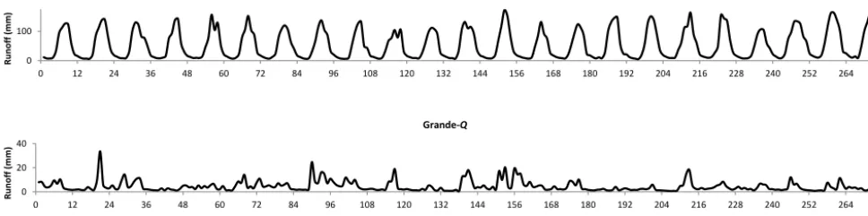
[image:3.612.57.541.77.197.2]Month Grande-Q
Figure 1. Schematic representation of different levels of recurrence in runoff (Q) time series from Mekong and Grande river basins.
cal. The recurrence of runoff and the other three hydrological variables are of high importance for a water management per-spective. For example, Fig. 1 compares monthly runoff from two different basins with high and low recurrence character-istics. Although total runoff volume and the seasonality are obviously dominant factors for water resource management, and therefore many previous classification studies have fo-cused on these metrics to represent them (Weingartner et al., 2013), anthropogenic systems have already adapted to the lo-cal hydrologilo-cal regimes to some extent. Generally, it is more challenging for water managers to handle a random pattern with high fluctuations and different from past experiences, such as floods and droughts happening at unexpected mag-nitudes in unexpected seasons. The feature of our proposed classification is to show which variables are recurrent or non-recurrent and how different combinations of the recurrence (i.e., our proposed river basin classes) are distributed in the world.
Section 2 describes the data used in this study, followed by the methodology to calculate recurrence and classifica-tion of large river basins in the world in Sect. 3. Secclassifica-tion 4 presents the results and regional characteristics of the basins. In Sect. 5, we discuss the relationship between our classi-fication and other metrics including aridity, seasonality and phasing between water and energy cycles, as well as future application of the proposed classification.
2 Data
This study uses the WATCH Forcing Data for the 20th Cen-tury (WFD) and the WATCH 20th CenCen-tury Model Output from the Water Model Intercomparison Project (WaterMIP) data sets provided by EU-WATCH. The forcing data are based on the European Centre for Medium Range Weather Forecasting (ECMWF) reanalysis ERA-40 data (Weedon et al., 2010, 2011). The model output data set represents con-temporary naturalized conditions, with no human interaction such as reservoirs or agricultural withdrawals at 0.5◦spatial resolution (Haddeland et al., 2011). The EU-WATCH project
includes land surface models (LSMs) and global hydrolog-ical models (GHMs) depending on models solving energy balance or not.
1. Precipitation: precipitation is provided as part of the WFD data set. LSMs require input rainfall and snowfall independently provided by the WFD data set, whereas GHMs use their own algorithms to separate rainfall and snowfall, using total precipitation as input. Since the partitions within the GHMs are not available in the pro-vided EU-WATCH data set, this study used total precip-itation for the classification as the aggregated variables of rainfall and snowfall.
2. Evaporation: simulated evaporation for each model is provided as total flux without the distinction of its source (transpiration from vegetation, bare soil evapo-ration, sublimation, etc.).
3. Runoff: simulated surface and subsurface runoff for each model are provided independently. However, since the partitions between surface and subsurface differ sig-nificantly among models total runoff is used in this study. River discharge is also provided for some mod-els but for comparative purposes generated runoff from land surface is selected for the classification.
0.0o 5.0o 23.5o 23.5o 35.0o 55.0o 35.0o 55.0o 0.0o 5.0o 23.5o 23.5o 35.0o 55.0o 35.0o 55.0o 1
No. Basin No. Basin No. Basin No. Basin No. Basin
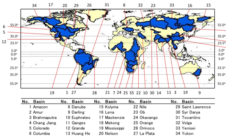
1 Amazon 8 Danube 15 Kolyma 22 Nile 29 Saint Lawrence
2 Amur 9 Darling 16 Lena 23 Ob 30 Syr Darya
3 Brahmaputra 10 Euphrates 17 Mackenzie 24 Okavango 31 Tocantins
4 Chang Jiang 11 Ganges 18 Mekong 25 Orange 32 Volga
5 Colorado 12 Grande 19 Mississippi 26 Orinoco 33 Yenisei
6 Columbia 13 Huang He 20 Nelson 27 La Plata 34 Yukon
7 Congo 14 Indus 21 Niger 28 Sao Francisco 35 Zambezi
2 3 4 5.0o 5.0o 5 6 7 8 9
10 11
12 3
14 15 16 17 19 20
21 22
23
24 25 26
27 28
29
30
31 32 33
34
[image:4.612.100.498.63.304.2]35 19
Figure 2. Location of the basins included in the analysis with an assigned identification number. The latitude reference lines identify the
latitudes that divide each of the regions geographically separating the basins.
3 Methods
3.1 Quantifying recurrence
This section introduces three metrics for evaluating recur-rence, which include AC, fast Fourier transform (FFT inten-sity) intensity and Colwell’s index of contingency (Colwell, 1974). In this study, since our interest is the recurrence of monthly variable as defined above, we used a period of 12 months for each metric. The definitions are described below and their characteristics are discussed in Sect. 5.2.
3.1.1 Lagged autocorrelation
A serial AC defined as (Eq. 1) describes the correlation of a time series with time lagk:
rk= N−k
P
i=1
(xi− ¯x) (xi+k− ¯x) N
P
i=1
(xi− ¯x)2
, (1)
whererk is the AC coefficient for lagk,N is the total num-ber of observations andx¯ is the mean. This AC calculation loses intensity as the lag increases dying down to zero as it approachesN. The AC can further be calculated in terms of the covariance but this computation is considered as a bias calculation of AC. In order to avoid the biased calculation and still be able to calculate a correlation between partial series with larger lags, this series can be assumed as a to-tally separate series with different mean and variance and the
calculations can be computed as simple correlation with the following equation
rk=
N−k
P
i
xi− ¯x[i,N−k] xi+k− ¯x[i+k,N]
"
N−k
P
i
xi− ¯x[i,N−k]2 #1/2"
N
P
i+k
xi+k− ¯x[i+k,N]2
#1/2. (2)
For the recurrence measure with monthly time series, eval-uating the AC of time lag 12 only is insufficient because it would only take into account the recurrence in contiguous years. We find it more appropriate to include the AC at other multiples of 12. Given the length of the time series used in this study, we decided to use the mean of AC from time lags 12, 24, 36, 48 and 60.
The results will be dependent also on the temporal resolu-tion (e.g., daily or yearly time series). However, in this study we decided to use a monthly resolution and look at yearly cy-cles because 1 year is usually a unit at which most of human activities and natural cycles repeat themselves.
3.1.2 Fast Fourier transforms
The other metric tested in this study is the FFT inten-sity which can identify important periods based on a pe-riodogram. The periodical part of a time series can be de-scribed by the following equation
mτ =µ+
h X
i=1
Aicos 2π iτ
p
+Bisin 2π iτ
p
wheremτis the harmonically fitted mean,µis the population mean, Ai andBi are the Fourier coefficients,p is a period (12 for monthly data) andhis the total number of harmonics (usuallyp/2).
The Fourier coefficients are calculated as
Ai =
2
p
p X
τ=1
¯
xτcos
2
π iτ p
, (4)
Bi= 2
p
p X
τ=1
¯
xisin 2π iτ
p
. (5)
The intensity can be calculated from these parameters as
Ii=A2i +B
2
i. (6)
The FFT intensity is important for identifying the periodicity at a particular frequency. A peak in the plot of intensity vs. frequency (periodogram) identifies a frequency for which a periodical pattern is found. For most hydrological data a peak at a frequency equivalent to a year exists (i.e., 12 months for monthly data, 52 weeks for weekly, and 365 for daily). If a series follows a pattern similar to a sinusoidal function, the intensity will be higher than a series departing from this pat-tern. Additionally, if a series contains much noise the inten-sity will also be reduced. Hence, a recurrent pattern shows higher FFT intensity. Since the FFT intensity is sensitive to the amplitude and magnitude we applied a standard normal-ization. Discussion on the characteristics and capability of FFT to measure recurrence is provided in Sect. 5.2
3.1.3 Colwell’s contingency index
Colwell (1974) introduced the indices of constancy and con-tingency, which together form the index called predictability. These indices have been used to analyze physical and biolog-ical temporal fluctuations. The index has been used widely in the analysis of flowering trees (Colwell, 1974), variations in river temperature (Vannote and Sweeney, 1980), variations in flow velocity (Riddell and Leggett, 1981), rainfall distri-bution at a yearly basis (Miller, 1984), periodicity analysis in streamflow or rainfall data (Gan et al., 1991), classification of flow regimes for environmental flow assessments (Zhang et al., 2012) and description of waterholes in hydrological regimes (Webb et al., 2012). Colwell (1974) defined pre-dictability as the measure of the certainty of knowing a state at a given time, being composed of the sum of two compo-nents: constancy, which represent how uniform the state of a variable is at different time cycles, and contingency, which measures the degree to which state and time are dependent on each other.
Calculation of the Colwell’s index requires first categoriz-ing the continuous data to prepare a matrix. The columns of the matrix represent time categories and rows represent the states of a phenomenon. In this study the columns represent different months and the rows represent ranges of standard deviations, whose ranges are between±4, which is equally divided into 16 categories with intervals of 0.5σ.
Now letNij be the number of times that a variable falls in stateiat time stepj. The sum of all columns for each statei
isXi, the sum of all rows for each time stepj isYi and the total number isZ. Then contingency (M) of Colwell’s index is defined as
M=H (X)+H (Y )−H (XY )
logs , (7)
wheresis the number of rows,H (X), H (Y) andH (XY) are defined as
H (X)= −X
j
Xj
Z log
Xj
Z , (8)
H (Y )= −X
i
Yi
Zlog
Yi
Z, (9)
H (XY )= −X
i X j Nij Z log N ij
Z . (10)
Contingency becomes 1 if a variable is at the same state at a particular time step, while the index becomes 0 if the oc-currences in different time steps take place at the same state. Contingency will be higher as more occurrences in a par-ticular time happen in a parpar-ticular state. If the values of a variable in a given month are similar, they will fall under the same state interval. This will be the case of variables with high recurrence. Further discussion on the capacity of Col-well’s index to represent the concept of recurrence is stated in Sect. 5.2. For reference, the constancy (C) and predictabil-ity (Pd) are defined as
C=1−H (Y )
logs , (11)
Pd=1−
H (XY )−H (X)
logs . (12)
3.2 Hydrological classification
High Recurrence
Runoff
Low Recurrence
Runoff
High Recurrence
Precip
Low Recurrence
Precip
High Recurrence
Precip
Low Recurrence
Precip
High Recurrence Storage
Low Recurrence Storage High Recurrence
Evap
Low Recurrence Evap
High Recurrence Evap
Low Recurrence Evap
High Recurrence Evap
Low Recurrence Evap
High Recurrence Evap
Low Recurrence Evap
High Recurrence Storage
Low Recurrence Storage
High Recurrence Storage
Low Recurrence Storage
High Recurrence Storage
Low Recurrence Storage
High Recurrence Storage
Low Recurrence Storage
High Recurrence Storage
Low Recurrence Storage
High Recurrence Storage
Low Recurrence Storage
High Recurrence Storage
Low Recurrence Storage
QPES
QPE
QPS
QP
QES
QE
QS
Q
PES
PE
PS
P
ES
E
S
[image:6.612.114.483.69.445.2]L
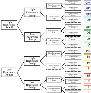
Figure 3. Hydrological classification tree. Color codes indicate the colors used in further maps to identify the classes to which basins belong.
Dashed lines indicate paths into classes that were not found in the studied basins.
classification tree in Fig. 3. The figure shows the 16 possible classes, and the combinations that were found and not within the basins of this study. It is provided to be used as a guidance to understand further figures. We used runoff as the first vari-able for the classification as it is the main concern for water resource management, and the other three variables are fur-ther used to explain why the runoff in each basin or region shows high or low recurrence. The value used for classifying the basins as high or low recurrence was an AC of 0.75.
First we quantified recurrence at global scale except for Greenland, where model performance was questionable due to its particular conditions, and Antarctica, where the EU-WATCH product was not cover. This global analysis was per-formed for the given time series of each variable at each in-dividual grid. The analysis for the world’s largest 35 basins was performed for the time series of each variable consider-ing the spatial average of the grids included within the limits of the basin.
Among all the model output from EU-WATCH, we paid particular attention to the WaterGAP model results because it is the only model that includes a calibration module and is closest to observations (Haddeland et al., 2011). Meanwhile, all other model results are also analyzed to cover different model behaviors and discuss model uncertainty (Sect. 5).
4 Results
dis-5.0o 23.5o 23.5o 35.0o 55.0o 35.0o 55.0o 5.0o 0.0o 5.0o 23.5o 23.5o 35.0o 55.0o 35.0o 55.0o 5.0o 0.0o 5.0o 23.5o 23.5o 35.0o 55.0o 35.0o 55.0o 5.0o 0.0o 5.0o 23.5o 23.5o 35.0o 55.0o 35.0o 55.0o 5.0o 0.0o 5.0o 23.5o 23.5o 35.0o 55.0o 35.0o 55.0o 5.0o 0.0o 5.0o 23.5o 23.5o 35.0o 55.0o 35.0o 55.0o 5.0o 0.0o 5.0o 23.5o 23.5o 35.0o 55.0o 35.0o 55.0o 5.0o 0.0o 5.0o 23.5o 23.5o 35.0o 55.0o 35.0o 55.0o 5.0o 0.0o Precipitation
a) b) Evaporation
Storage
c) d) Runoff
Autocorrelation
[image:7.612.59.538.66.323.2]0.50 0.75 1.00 -0.10
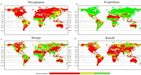
Figure 4. Recurrence in main hydrological variables at global scale: (a) precipitation, (b) evaporation, (c) storage and (d) runoff. The map
identifies the areas with lowest recurrence (<0.5), low recurrence (0.5–0.75) and high recurrence (0.75<). Reference latitude lines identify the divisions in latitudinal regions where particular conditions and similarities were found to exist.
tribution maps of the recurrence (i.e., AC in this case) in the four variables: precipitation, evaporation, storage and runoff. From the recurrence calculated for each variable’s time se-ries, each grid was identified with red for very low recurrence (<0.5), yellow for low recurrence (0.5–0.75) and green for high recurrence (0.75–1.0). To explain the distribution of the recurrences in the four variables, this paper uses the follow-ing terms for different latitude zones for both hemispheres: tropical (0–23.5◦), subtropical (23.5–35◦), temperate (35– 55◦) and sub-arctic and Arctic (55–90◦).
The precipitation in the tropical region is basically charac-terized by the seasonality caused by the oscillation of the in-tertropical convergence zone (ITCZ), and energy supply due to the effects of the Earth’s tilt fluctuation. Because of this seasonality, two bands between 5 and 23.5◦for both hemi-spheres show high recurrence in all variables, while they are lower in general at the equatorial band between 5◦S and 5◦N
where there is no seasonality. The rest of the variables fol-low generally the same pattern as precipitation although the high recurrence areas of storage and runoff are comparatively smaller than that of precipitation.
The subtropical region is mainly characterized by the lat-itudinal desert belts. This region is characterized by low hu-midity and general dryness in soil conditions. In this region, precipitation events are typically sudden and intense without following certain temporal patterns. During rainfall events the other variables also behave similarly. Hence, all of the four variables tend to have low recurrence. The Southeast
Asia monsoon area is an exception since its behavior is simi-lar to the humid tropics area, therefore displaying high recur-rence in all variables.
The temperate region also shows generally low recurrence in precipitation due to continental climates or oceanic cli-mates with no dry season. Eastern Asia is the only region showing high recurrence due to the effects of the Asian mon-soon. Evaporation in this region has high recurrence due to seasonality with the exception of dry areas in Europe and Asia. Storage has different geographic patterns throughout the region. Runoff follows the same regionalization as stor-age except for Europe with comparatively low recurrence in general.
Precipitation in the sub-arctic and arctic region shows low recurrence except for some areas in North America and east-ern Siberia. Evaporation exhibits the higher recurrence in this area. The extent area of high recurrence in storage and runoff is larger in this region mainly attributed to the amount of snow.
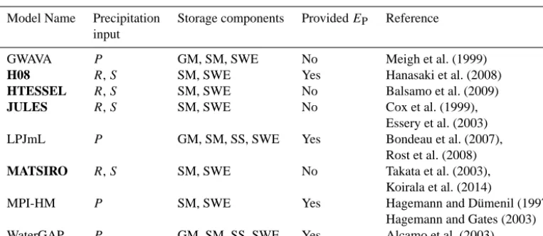
Table 1. Overview of models included in this research and their characteristics. Adapted from Haddeland et al. (2011) and Gudmundsson
et al. (2012a, b). Model names in bold are considered as LSMs. Precipitation input is either provided as total precipitation (P) or as rainfall (R) and snowfall (S) separately. Storage can be handled in models as ground moisture (GM), soil moisture (SM), surface storage (SS) and snow water equivalent (SWE). Potential Evaporation (EP) is provided (yes) or not provided (no).
Model Name Precipitation Storage components ProvidedEP Reference input
GWAVA P GM, SM, SWE No Meigh et al. (1999)
H08 R,S SM, SWE Yes Hanasaki et al. (2008)
HTESSEL R,S SM, SWE No Balsamo et al. (2009)
JULES R,S SM, SWE No Cox et al. (1999),
Essery et al. (2003)
LPJmL P GM, SM, SS, SWE Yes Bondeau et al. (2007),
Rost et al. (2008)
MATSIRO R,S SM, SWE No Takata et al. (2003),
Koirala et al. (2014)
MPI-HM P SM, SWE Yes Hagemann and Dümenil (1997),
Hagemann and Gates (2003)
WaterGAP P GM, SM, SS, SWE Yes Alcamo et al. (2003)
GWAVA: Global Water Availability Assessment; HTESSEL: Hydrology-Tiled ECMWF Scheme for Surface Exchange over Land; JULES: Joint UK Environment Simulator; LPJmL: Lund–Potsdam–Jena managed Land; MATSIRO: Minimal Advanced Treatments of Surface Interaction and Runoff; MPI-HM: Max Planck Institute – Hydrology Model; WaterGAP: Water – Global Assessment and Prognosis.
0.0o
5.0o
23.5o
35.0o
55.0o
5.0o
23.5o
35.0o
55.0o
0.0o
5.0o
23.5o
35.0o
55.0o
5.0o
23.5o
35.0o
55.0o
QPES QPE QPS
QES QE
PES PE
ES E
L
Figure 5. Basin location map with identification by class. A threshold for defining high recurrence or low recurrence was set at 0.75.
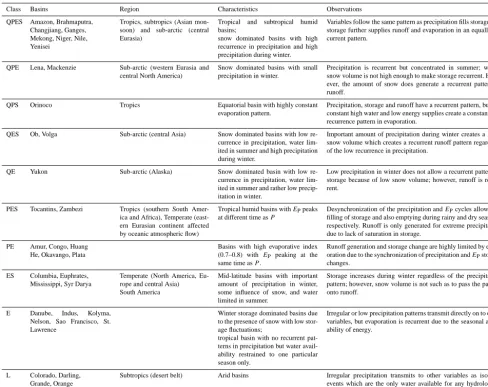
[image:8.612.58.538.403.649.2]Table 2. Summary of class characteristics.
Class Basins Region Characteristics Observations
QPES Amazon, Brahmaputra, Changjiang, Ganges, Mekong, Niger, Nile, Yenisei
Tropics, subtropics (Asian mon-soon) and sub-arctic (central Eurasia)
Tropical and subtropical humid basins;
snow dominated basins with high recurrence in precipitation and high precipitation during winter.
Variables follow the same pattern as precipitation fills storage and storage further supplies runoff and evaporation in an equally re-current pattern.
QPE Lena, Mackenzie Sub-arctic (western Eurasia and central North America)
Snow dominated basins with small precipitation in winter.
Precipitation is recurrent but concentrated in summer; winter snow volume is not high enough to make storage recurrent. How-ever, the amount of snow does generate a recurrent pattern in runoff.
QPS Orinoco Tropics Equatorial basin with highly constant evaporation pattern.
Precipitation, storage and runoff have a recurrent pattern, but the constant high water and low energy supplies create a constant low recurrence pattern in evaporation.
QES Ob, Volga Sub-arctic (central Asia) Snow dominated basins with low re-currence in precipitation, water lim-ited in summer and high precipitation during winter.
Important amount of precipitation during winter creates a large snow volume which creates a recurrent runoff pattern regardless of the low recurrence in precipitation.
QE Yukon Sub-arctic (Alaska) Snow dominated basin with low re-currence in precipitation, water lim-ited in summer and rather low precip-itation in winter.
Low precipitation in winter does not allow a recurrent pattern in storage because of low snow volume; however, runoff is recur-rent.
PES Tocantins, Zambezi Tropics (southern South Amer-ica and AfrAmer-ica), Temperate (east-ern Eurasian continent affected by oceanic atmospheric flow)
Tropical humid basins withEPpeaks at different time asP
Desynchronization of the precipitation andEPcycles allows for filling of storage and also emptying during rainy and dry seasons, respectively. Runoff is only generated for extreme precipitation due to lack of saturation in storage.
PE Amur, Congo, Huang He, Okavango, Plata
Basins with high evaporative index (0.7–0.8) with EP peaking at the same time asP.
Runoff generation and storage change are highly limited by evap-oration due to the synchronization of precipitation andEPstorage changes.
ES Columbia, Euphrates, Mississippi, Syr Darya
Temperate (North America, Eu-rope and central Asia) South America
Mid-latitude basins with important amount of precipitation in winter, some influence of snow, and water limited in summer.
Storage increases during winter regardless of the precipitation pattern; however, snow volume is not such as to pass the pattern onto runoff.
E Danube, Indus, Kolyma, Nelson, Sao Francisco, St. Lawrence
Winter storage dominated basins due to the presence of snow with low stor-age fluctuations;
tropical basin with no recurrent pat-terns in precipitation but water avail-ability restrained to one particular season only.
Irregular or low precipitation patterns transmit directly on to other variables, but evaporation is recurrent due to the seasonal avail-ability of energy.
L Colorado, Darling, Grande, Orange
Subtropics (desert belt) Arid basins Irregular precipitation transmits to other variables as isolated events which are the only water available for any hydrological process to take place.
L is low recurrence in all variables.
recurrence calculated using the other models. Table 2 sum-marizes the characteristics of each class.
4.1 Tropical region (0.0–23.5◦)
The tropical region has the most diversity of classes. In this region we found basins belonging to the QPES, QPS, PES, PE and E classes. Mainly, there are two distinct patterns observed in runoff. High recurrence in runoff takes place in the most humid basins exemplified in Fig. 7a by QPES and Fig. 7b by QPS. Consistent with the global analysis re-sults, we found that precipitation is highly recurrent for these classes due to a repeating pattern resulting from the oscilla-tion of the ITCZ. Evaporaoscilla-tion and storage are also highly recurrent as they follow the same pattern as precipitation, as can be seen in the Amazon time series in Fig. 8a. In the Orinoco Basin evaporation is maintained rather constant as the basin is energy limited and potential evaporation is
con-stant resulting in low recurrence in evaporation. Storage on the other hand follows the same pattern as precipitation re-sulting in a highly recurrent pattern.
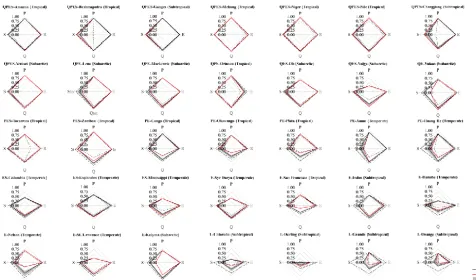
Figure 6. Radar charts depicting the results of recurrence for each variable in each individual basin. Results from the WaterGAP model are
highlighted in red, the model mean is shown as a solid black line, the interquartile is shaded in gray, and the max. and min. values are shown with a dashed black line.
dry season (Fig. 8c and storage component climatology of Zambezi Basin in the Supplement). This creates a strong sea-sonal pattern in total storage leading to high recurrence. The PE class is characterized by the peaks of potential evapora-tion andP peaking at the same time (Fig. 7d: PE). Compared to Amazon, average precipitation is much lower but poten-tial evaporation is almost the same. The Congo Basin can be energy limited (P > ET−EP) in the wet season; therefore,
regardless of the amount of precipitation, evaporation will reach its potential creating a more recurrent pattern in evap-oration. The anomalies in precipitation directly transfer to storage and runoff variations, and since runoff ratio (Q/P) and storage change ratio (1S/P) are much smaller, these anomalies are larger relative fluctuations to these variables; hence, recurrence in storage and runoff patterns is low. Sao Francisco Basin is an exception in this region consisting only of recurrent evaporation. This type of basin is mainly seen in the temperate region and is explained in detail in Sect. 4.3. 4.2 Subtropical region (23.5–35.0◦)
In subtropical region, mainly two patterns of classes are ob-served. On the one hand, QPES river basins are located in Southeast Asian monsoon, where similar behaviors are ob-served as the same class river basins in tropical region. On the other hand, we can observe the basins that are extremely dry, represented by Orange Basin in Fig. 7. In the latter basins, all
variables follow the patterns of precipitation being, sudden, abrupt and lacking any defined temporal distribution, leading to class L (i.e., none of the variables are recurrent). The Indus River basin is an exception in this region belonging to the E class.
4.3 Temperate region (35.0–55.0◦)
In the temperate region there are three particular classes ob-served: PE, ES and E. All of these classes have low recur-rence in runoff and high recurrecur-rence in evaporation due to the seasonality in energy supply.
Basins located in eastern Asia belong to the PE class as explained previously in the tropical region section. The rea-sons why this class takes place in the temperate region are the same as that for the tropical region, i.e., the reason for re-currence in precipitation is coming from the moisture supply following the Asia monsoon pattern.
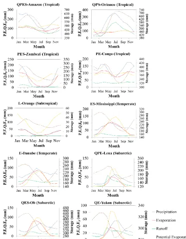
Figure 7. Variable climatologies for selected basins for each class and region. The charts present a particular basin for each of the 10 classes
found sorted by region. Comparable axis of precipitation, evaporation, runoff and potential evaporation are shown on the left vertical axis and storage axis is shown on the right vertical axis.
to decrease. In these basins there is some influence of snow; however, the amount of snow is not as high enough to create a recurrent runoff pattern.
Another group in the temperate region is characterized by recurrence in evaporation only as is exemplified by the Danube River basin. In these basins, precipitation has a pat-tern of low recurrence that transfers to the variables of stor-age and runoff. As compared to the Mississippi, the Danube River basin is not energy limited during summer. This
cre-ates a pattern whereby the anomalies and low recurrence of precipitation also transfer to storage thereby reducing its re-currence.
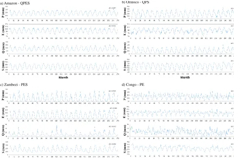
en-a) Amazon - QPES b) Orinoco - QPS
c) Zambezi - PES d) Congo - PE
AC=0.892
AC=0.679
AC=0.870
AC=0.878 AC=0.897
AC=0.921
AC=0.860
AC=0.904
AC=0.925
AC=0.966
AC=0.612
AC=0.856
AC=0.829
AC=0.861
AC=0.404
[image:12.612.59.539.66.390.2]AC=0.696
Figure 8. Monthly time series of selected basins in the tropics from each class: (a) Amazon – QPES, (b) Orinoco – QPS, (c) Zambezi – PES, (d) Congo – PE. The graphs exemplify time series with high or low recurrence depending on the classification. The averaged AC coefficient
is provided in the top right corner of each graph.
Table 3. Component contribution ratio (CCR) for basins located in
the sub-arctic region. The CCR is calculated as in Kim et al. (2009).
Basin Ground moisture Soil moisture Surf storage SWE
Yenisei 0.056 0.095 0.247 0.602
Lena 0.021 0.076 0.391 0.512
Mackenzie 0.077 0.135 0.109 0.679
Ob 0.077 0.225 0.112 0.586
Volga 0.083 0.271 0.145 0.501
Yukon 0.059 0.052 0.312 0.577
Kolyma 0.011 0.034 0.322 0.633
ergy supply. All of the basins in this region except Kolyma have recurrent runoff. The runoff pattern is dominated by snowmelt taking place similarly year after year as observed in the sudden peak in runoff during spring (Fig. 7h–j).
Basins belonging to the QPES and QPE classes have high recurrence in precipitation due to moisture inflow from the ocean (Figs. 4a and 5). The recurrence in storage is de-pendent on the amount of snow. The climatologies of these basins (Fig. 7h–j) show that storage peaks during the win-ter months due to the accumulation of snow. Figure 9 shows
the climatology of storage in these basins further subdivided into the volume of the different components. Table 3 shows the component contribution ratio (CCR) (Kim et al., 2009) describing the contribution of each storage variation to the variation of total storage. As it can be seen, in these basins the highest contribution takes place from snow. The Water-GAP model in particular has a small groundwater tank which includes only the dynamical part making it small in volume and contribution. Figures 10 and 11 show the snow water equivalent (SWE) and seasonal precipitation amounts. From these two figures, we can observe that basins with higher snow accumulation have higher recurrence both in storage and runoff.
[image:12.612.49.283.484.568.2]Figure 9. Climatology of storage and the various storage
compo-nents for sub-arctic basins.
0 20 40 60 80 100 120 140
Jan Feb Mar Apr May Jun Jul Aug Sep Oct Nov Dec
SWE
V
o
lum
e
(m
m
)
QPES-Yenisei QES-Ob QES-Volga QPE-Lena QPE-Mackenzie QE-Yukon E-Kolyma
Figure 10. Snow water equivalent seasonality of sub-arctic basins.
5 Discussion
5.1 Characteristics of recurrence measured by AC 5.1.1 Recurrence vs. seasonality
This section discusses the characteristics of recurrence mea-sured by AC from monthly variables with the lags of 12 month multiples. First, we compare the recurrence and seasonality, following the definition of Walsh and Lawler
0 50 100 150 200 250
DJF MAM JJA SON
Pr
eci
pita
tion
(mm) QPES-Yenisei
QES-Ob
QES-Volga
QPE-Lena
QPE-Mackenzie
QE-Yukon
[image:13.612.305.549.68.219.2]E-Kolyma
Figure 11. Seasonal precipitation climatology of sub-arctic basins.
(1981): SI= 1
R 12 X
n=1
x¯n− ¯R/12
, (13)
[image:13.612.47.288.427.551.2]wherex¯nis the mean rainfall of monthnandR¯is the annual mean of a hydrological variable. Hence, the seasonality mea-sures the degree to which each monthly variable of a regime curve deviates from the overall annual mean. Seasonality is essentially different from the recurrence which, as defined above, measures the degree to which a monthly hydrolog-ical variable returns to the same state in subsequent years. Figure 12 displays the relationship between recurrence and seasonality for all the time series in the study, including each variable from every basin. The figure suggests that generally higher seasonal variability tends to have higher recurrence. This is because if a variable has strong seasonality, the influ-ence of the deviation from the climatology has comparatively less impact on the AC. Appendix A shows the distribution of seasonality and recurrence in all variables.
Nevertheless, there are exceptions where variables are highly seasonal but not recurrent. For example, Fig. 13 shows the monthly average precipitation in Ob and Yenisei. The two basins are located in the same latitudinal region sharing their borders. The climatologies of the both basins are similar with comparable magnitudes at all months. However, the year to year variability in the both basins are different: Ob shows higher variations than Yenisei. Therefore, the precipitation in Ob has lower recurrence (0.65) than that in Yenisei (0.88). Similar cases can be observed when comparing the clima-tologies shown in Fig. 7 and the measure of recurrence pre-sented in Fig. 6, and in previous work (e.g., Kim et al., 2009) where storage climatologies show strong seasonality but the yearly time series does not behave in a recurrent manner.
R² = 0.24
0 0.1 0.2 0.3 0.4 0.5 0.6 0.7 0.8 0.9 1
-0.2 0 0.2 0.4 0.6 0.8 1
Sea
so
na
lity
[image:14.612.307.550.65.349.2]Recurrence (AC)
Figure 12. Relationship between recurrence and seasonality from
all of the time series corresponding to each variable in each basin.
recurrence. Case 3 and case 4 are precipitation of Yenisei and Ob with similar seasonality and high recurrence in Yeni-sei and low recurrence in Ob as discussed above. Case 5 is a sinusoidal pattern repeating the exact same values and show high seasonality and recurrence. Case 6 adds a decreasing trend to the case 5, but it keeps similar seasonality and recur-rence. In summary, seasonality is calculated from the clima-tology of a variable which results from a long-term average, while recurrence measures the year to year variability of the monthly pattern of a variable. Recurrence is an additional feature of temporal patterns of basins providing different in-formation than seasonality.
5.1.2 Recurrence vs. aridity
Recurrence in runoff and storage also has some relation with the aridity of a basin as well as the timings of energy and water availability. These basin characteristics are essential in determining the basins’ functionality as they are a descrip-tor of how much water from precipitation is transferred to evaporation, storage change or runoff, and they have been included as classification indices in previous works such as Jothityangkoon and Sivapalan (2009), Coopersmith et al. (2012, 2014) and Berghuijs et al. (2014). Figure 15 shows the relations between aridity, timing of peaks in precipita-tion (water supply) andEP (energy supply) with recurrence
in runoff and precipitation by region.
[image:14.612.48.290.68.209.2]Figure 15a and b show that in humid basins, where the runoff ratio and the storage change ratio are high, runoff and storage follow the patterns in precipitation. Drier basins have low recurrence in runoff (classified as PES, PE, ES or E), es-sentially due to the high sensitivity of runoff to precipitation under smaller runoff ratios. For example, the case of Amazon and Congo, aforementioned in Sect. 4.1, has a difference in recurrence of storage and runoff. For precipitation, both vari-ables have similar relative variations but the total precipita-tion in Congo is about 70 % of the precipitaprecipita-tion in Amazon. Additionally, the runoff ratio is smaller in Congo (0.4) than
Figure 13. Seasonal climatologies of precipitation in Yenisei and
Ob river basins (a), long-term mean (b), and (c) 23-year precipita-tion in Yenisei and Ob river basins. (b) and (c) show the minimum, maximum quartiles and mean for each month.
in Amazon (0.45). The physical meaning of this aspect is that there is less water volume in Congo transferring from precip-itation into storage fluctuation and runoff generation. Hence, the same anomalies in precipitation have a larger impact in Congo than in Amazon. Furthermore, recurrence of storage and runoff also depends on the timing ofP andEPpeaks. As
Fig. 15c and d indicate, the recurrence becomes higher ifP
andEPare out of phase (>2 months).
5.2 Recurrence measured by FFT intensity and Colwell’s contingency compared to AC
Table 4. Results of Colwell’s indices (constancy –C, contingency – Mand predictability –Pd) for all variables in arid basins. Constancy has high values due to variables being constantly low, increasing the total predictability index.
Basin Variable C M Pd
Colorado P 0.303 0.110 0.413
E 0.284 0.265 0.549
Q 0.433 0.115 0.548
S 0.302 0.209 0.511
Darling P 0.300 0.073 0.373
E 0.297 0.209 0.506
Q 0.380 0.179 0.559
S 0.291 0.170 0.461
Grande P 0.320 0.173 0.493
E 0.320 0.207 0.527
Q 0.432 0.089 0.521
S 0.297 0.077 0.374
Orange P 0.339 0.176 0.515
E 0.311 0.202 0.513
Q 0.507 0.067 0.574
S 0.365 0.077 0.442
at a particular time. For this reason Colwell’s contingency results are highly consistent with the results of AC and FFT intensity. Colwell’s contingency is not only consistent with the other indices but also adequate for measuring recurrence as defined above. Table 5 shows the classification of each basin using the different metrics.
Figure 16 shows the correlation between AC and FFT in-tensity and AC and Colwell’s contingency from the Water-GAP model. All indices correlate well although there are par-ticular cases that deviate from the regressions. As mentioned in the methodology section, the threshold selected for AC was 0.75. For FFT intensity and Colwell’s contingency mea-sures thresholds of 150 and 0.25 were selected to minimize the number of basins categorized as different classes. Table 5 shows the classification of basins from different metrics.
[image:15.612.74.258.118.316.2]The FFT procedure is used to represent a time series by fit-ting a sine and cosine function; therefore, the FFT intensity will be higher for variables following a sinusoidal pattern. Figure 17 exemplifies the different periodogram with their respective partial time series and climatology. Figure 17a shows the example of evaporation in Changjiang for which a highly sinusoidal pattern indicates high AC and FFT inten-sity. Figure 17b shows an example of low recurrence with low AC and FFT intensity. However there are two examples where the FFT intensity value indicates low recurrence while AC indicates high recurrence. First, Fig. 17c (Congo evapo-ration) shows a bimodal pattern which has a high AC but low FFT intensity; since the peaks in evaporation appear at dif-ferent frequencies, the intensity at a period of 12 months be-comes weaker and other high intensities appear at different frequencies. The second example shown in Fig. 17d, takes
Table 5. Classification using different metrics, autocorrelation
(AC), Colwell’s contingency (M) and fast Fourier transforms (FFT).
Basin AC M FFT
Amazon QPES QPES QPES
Amur QPE QPE QPE
Brahmaputra QPES QPES QPES
Changjiang QPES QPES QPES
Colorado L E S
Columbia ES ES ES
Congo PE PE L
Danube E E ES
Darling L L L
Euphrates ES PES QPES
Ganges QPES QPES PES
Grande L L L
Huanghe PE PE PE
Indus E E L
Kolyma E QE E
Lena QPE QPE PE
Mackenzie QPE QPE PES
Mekong QPES QPES QPES
Mississippi ES ES ES
Nelson E E PES
Niger QPES QPES QPES
Nile QPES QPES QPES
Ob QES QES ES
Okavango PE PE PE
Orange L L L
Orinoco QPS QPS QPES
Plata PE PE PES
Sao Francisco E E PES
St. Lawrence E E ES
Syr Darya ES ES ES
Tocantins PES PES QPES
Volga QES QES ES
Yenisei QPES QPES PES
Yukon QE QE QE
Zambezi PES PES PES
place with basins in the sub-arctic region where the highest volume in runoff comes from snowmelt in early spring, but the peak in precipitation takes place during summer, creat-ing a lump in the recession of the runoff climatology. This second lump reduces the intensity at a period of 12 months and increases other frequencies seen on the periodogram. For both of these cases with deviations from a sinusoidal func-tion, AC better represents the concept of recurrence because if the same pattern repeats, independent of the shape of the pattern, AC at lag multiples of 12 will be higher.
in-Case Seasonality Standard
[image:16.612.128.469.63.580.2]Deviation Recurrence (AC) Case 1 0.031 0.14 1.000 Case 2 0.242 2.53 0.093 Case 3 0.410 2.15 0.843 Case 4 0.410 2.22 0.690 Case 5 0.622 2.82 1.000 Case 6 0.789 3.38 1.000
Figure 14. Schematic time series representing different levels of recurrence, variability and seasonality.
clude the dependence of the results on the amount of classes selected, and the tendency for higher values in contingency with shorter record lengths. These are the intrinsic limitations of Colwell’s index with the discretization of data.
5.3 Result dependency on model structure
Figure 15. Relation of Aridity and Timing of peaks and recurrence in runoff. (a) Timing of P andEPwith recurrence in runoff, (b) relation of timing of peaks in P andEPpeaks and recurrence in storage, (c) relation of aridity and recurrence in runoff., and (d) relation between aridity and recurrence in storage.
[image:17.612.58.540.534.695.2]a) Changjiang Evaporation
d) Yenisei Runoff c) Congo Precipitation
b) Orange Storage
AC=0.983 M=0.497 FFT intensity=191
AC=0.132 M=0.077 FFT intensity=77
AC=0.888 M=0.353 FFT intensity=142 AC=0.824
[image:18.612.58.540.68.262.2]M=0.299 FFT intensity=129
Figure 17. Examples of variables with different results in FFT intensity. (a) Changjiang’s evaporation, (b) runoff in Yenisei, (c) precipitation
in Congo and (d) storage in Orange.
recurrence. Figure 18 shows the box plots containing the ranges of recurrence for every variable in all basins by the eight different models.
Marginal differences on recurrence are found in most of the tropical humid basins in the QPES class. Larger differ-ences are observed in storage variables in these basins. For the case of the Brahmaputra GWAVA and the MPI-HM mod-els are outliers in the recurrence of storage computing 0.03 and 0.55, respectively, while other models range between 0.92 and 0.96. Haddeland et al. (2011) highlighted the over-estimation of evaporation in this basin by MPI-HM due to the use of the Thornthwaite evaporation scheme. This leads to higher interannual variations on storage components due to higher evaporation. In the case of GWAVA, the storage se-ries for this basin shows a cyclic increase in storage until it is abruptly decreased to a lower volume. This pattern is only observed in the snow component of storage which is highly overestimated in GWAVA as compared to other models. The MATSIRO model has a deep groundwater tank which in gen-eral generates less seasonal variation in runoff (Haddeland et al., 2011). This has an effect on the recurrence calculation and in many basins recurrence in runoff changes from high on all models to low in MATSIRO.
Models in the temperate zone show larger differences mostly in runoff and storage recurrence. This is due to the variety of climatologies that are present in this zone and the presence of snow. Snowfall is treated differently in each GHM, with different thresholds for snowfall, and among all models there are different melting schemes. These differ-ences mainly affect basins that are around the threshold zone between 0 and 1◦C where precipitation is partitioned
be-tween snow or rain and melting processes start (Haddeland et al., 2011). Despite these large differences, most models indicate the same class for most basins. In sub-arctic basins,
where the influence of snow is much more important, the differences are low but the WaterGAP represent the lowest recurrent pattern of all models. This is possibly due to the degree day method. Temporal and spatial variations in snow content are larger in the WaterGAP model decreasing recur-rence. However, the relation of storage recurrence and snow amount is kept as basins with higher snow content also ex-hibit higher recurrence.
Finally, arid basins have wide uncertainty due to the dif-ferences in partition between evaporation and runoff in each model. MATSIRO is an outlier in having high recurrence in evaporation. When inspecting the time series of storage for these catchments, a marked decreasing trend was found. This can be partially attributed to the deep groundwater tank that keeps water available for evaporation despite the lack of wa-ter supply through precipitation. Evaporation follows a sea-sonal cycle in MATSIRO with increasing recurrence.
QPES-Amazon PE-Amur QPES-Brahmaputra QPES-Changjiang L-Colorado
ES-Euphrates ES-Darling
E-Danube PE-Congo
ES-Columbia
QPES-Ganges L-Grande PE-Huang He E-Indus E-Kolyma
E-Nelson ES-Mississippi
QPES-Mekong QPE-Mackenzie
QPE-Lena
QPES-Niger QPES-Nile QES-OB PE-Okavango L-Orange
ES-Syr Darya E-St. Lawrence
E-Sao Francisco PE-Plata
QPS-Orinoco
[image:19.612.55.538.66.442.2]PES-Tocantins QES-Volga QPES-Yenisei QE-Yukon PES-Zambezi
Figure 18. Model differences. Box plots show the recurrence measure for each variable in each basin displaying an interquartile uncertainty
band, WaterGAP marked by the red spot, the mean highlighted by the black mark and the maximum and minimum values.
time lag due to the length of the river. Further analysis should be performed in order to understand the effects of the inclu-sion of river channel storage in the measures of recurrence. 5.4 Future application of the classification framework By deriving the classification framework based on recur-rence, we were able to discuss the interactions among the hy-drologic variables affecting their temporal pattern. As one of future applications of the proposed classification, we would like to analyze the impact of projected climate change on hydrologic variables depending on the classes in a mech-anistic way. A mechmech-anistic approach to analyze hydrolog-ical changes is climate elasticity quantification of runoff (Sankarasubramanian et al., 2001; Yang and Yang, 2011; Vano et al., 2012). We believe that sensitivity studies could be further enhanced with this kind of classification highlighting dominant hydrologic processes, especially by incorporating a storage component.
6 Conclusions
This paper presented a framework of hydrologic classifica-tion applicable to large-scale river basins based on monthly temporal variations of precipitation, evaporation, storage and runoff. The classification was derived from the concept of hydrological recurrence as a metric defined as the degree to which a monthly hydrological variable returns to the same state in subsequent years. The recurrence was measured us-ing the mean of autocorrelations (AC) with the multiples of 12 to 60 month lags, the intensity of fast Fourier transforms (FFT intensity) and Colwell’s contingency index. These mea-sures were calculated at global gridded scale (0.5◦) and at the 35 largest basins of the world based on the model forcing or output of the EU-WATCH data set.
The recurrence of individual variables is generally dif-ferent in difdif-ferent latitudinal regions. For the recurrence in precipitation, the seasonality of moisture plays an important role, while for that in evaporation, the effect of seasonality in energy is more dominant. Storage recurrence is more depen-dent on the seasonality of moisture in the tropics and snow at higher latitudes. Finally, all combinations control the charac-teristics of the recurrence in runoff.
According to our proposed classification, which results in 16 possible classes from the combinations of high or low re-currence of the four variables, only 10 classes are present from our study of river basins. In the tropical region, essen-tially recurrence in runoff and storage is dependent on arid-ity. Humid basins are highly recurrent in all variables. Drier basins have low recurrence in runoff, but storage recurrence is dependent on the timing of the peaks in precipitation and
EP.
In the temperate region, evaporation is always recurrent due to high seasonality, while precipitation shows low recur-rence in this region, due to basins’ aridity. In these basins, the timing of peaks betweenP andEPalso influence the
re-currence inQandS.
In the sub-arctic region, evaporation is again highly recur-rent due to extreme seasonality. Precipitation is recurrecur-rent in areas with oceanic currents influences. Recurrence in storage is in the basins with larger amounts of snow, whose melting processes dominate the patterns of runoff. As a result, the runoff recurrence is high in this region, while the storage re-currence varies in different areas. Therefore, the river basins are mainly classified into QPES, QPE, QES or QE depending on their combinations.
The above results were primarily obtained based on the analysis of AC metric with WaterGAP model output. How-ever, the other two metrics, FFT intensity and Colwell’s tingency, and other eight models also essentially showed con-sistent results.
Overall the presented approach is an attempt to define basin similarity accounting for the temporal patterns of wa-ter balance components. River basins in the different classes are likely to behave differently even under similar changes in climate control. The same framework may be applied to long-term time series data from different sources including GCM future projections. Furthermore, by using long-term time series broken down into partial time series, the proposed framework may identify a hydrologic regime shift from one class to another, as well as the characteristics of hydrologic sensitivity in different classes. For this kind of study, EU-WATCH provides useful data sets for projecting future hy-drologic variables.
Appendix A: Spatial comparison of recurrence and seasonality
Figure A1 shows the recurrence and seasonality for each variable in each basin. Precipitation shows high recurrence in most of South America, most of Africa, Southeast Asia, and the majority of basins in eastern Asia as displayed in Fig. A1a. In Fig. A1b, it can be noted that seasonality is not that strong for the majority of the basins, aside from a few basins in Africa and the Ganges in Southeast Asia. Fig-ure A1c and A1d show the recurrence and seasonality of evaporation, respectively. Evaporation is the most recurrent variable; however, the seasonality is low except for the sub-arctic basins. Runoff is mostly recurrent in some basins of the sub-arctic region and some basins in the tropics and South-east Asia (Fig. A1e), whereas it does not display seasonality except for in the Ganges and Lena basins (Fig. A1f). Finally, storage is a recurrent variable in some basins of South Amer-ica, Africa and Asia as can be seen from Fig. A1g. In the case of storage it does not display significant seasonality around
the world (Fig. A1h). Figure A1. (a) Recurrence of precipitation, (b) seasonality of pre-cipitation, (c) recurrence of evaporation, (d) seasonality of
The Supplement related to this article is available online at doi:10.5194/hess-19-1919-2015-supplement.
Acknowledgements. The authors would like to thank EU-WATCH
for making available the data set used in this study. We would also like to thank Pat J. F. Yeh for introducing the EU-WATCH and guiding in the initial stages of this research. Additionally we would also like to express our deepest gratitude to the two anonymous referees for their constructive comments and the handling editor Carlo De Michele and handling executive editor Alberto Guadagnini.
Edited by: C. De Michele
References
Alcamo, J., DÖLL, P., Henrichs, T., Kaspar, F., Lehner, B., RÖSCH, T., and Siebert, S.: Development and testing of the WaterGAP 2 global model of water use and availability, Hydrol. Sci. J., 48, 317–337, 2003.
Ali, G., Oswald, C. J., Spence, C., Cammeraat, E. L., McGuire, K. J., Meixner, T., and Reaney, S. M.: Towards a unified treshold based hydrological theory: necessary components and recurring challenges, Hydrol. Proc., 27, 313–318, 2013.
Balsamo, G., Beljaars, A., Scipal, K., Viterbo, P., van den Hurk, B., Hirschi, M., and Betts, A. K.: A revised hydrology for the ECMWF model: Verification from field site to terrestrial water storage and impact in the Integrated Forecast System, J. Hydrom-eteorol., 10, 623–643, 2009.
Berghuijs, W. R., Sivapalan, M., Woods, R. A., and Savenije, H. H. G.: Patterns of similarity of seasonal water balances: A window into streamflow variability over a range of time scales, Water Re-sour. Res., 50, 5638–5661, 2014.
Black, P. E.: Watershed functions, JAWRA J. Am. Water Resour. Assoc., 33, 1–11, 1997.
Bondeau, A., Smith, P. C., Zaehle, S., Schaphoff, S., Lucht, W., Cramer, W., Gerten, D., Lotze Campen, H., Müller, C., and Re-ichstein, M.: Modelling the role of agriculture for the 20th cen-tury global terrestrial carbon balance, Glob. Change Biol., 13, 679–706, 2007.
Cheng, L., Yaeger, M., Viglione, A., Coopersmith, E., Ye, S., and Sivapalan, M.: Exploring the physical controls of re-gional patterns of flow duration curves – Part 1: Insights from statistical analyses, Hydrol. Earth Syst. Sci., 16, 4435–4446, doi:10.5194/hess-16-4435-2012, 2012.
Colwell, R. K.: Predictability, constancy, and contingency of peri-odic phenomena, Ecology, 1148–1153, 1974.
Coopersmith, E., Yaeger, M. A., Ye, S., Cheng, L., and Sivapalan, M.: Exploring the physical controls of regional patterns of flow duration curves – Part 3: A catchment classification system based on regime curve indicators, Hydrol. Earth Syst. Sci., 16, 4467– 4482, doi:10.5194/hess-16-4467-2012, 2012.
Coopersmith, E., Minsker, B., and Sivapalan, M.: Patterns of re-gional hydroclimatic shifts: An analysis of changing hydrologic regimes, Water Resour. Res., 50, 1960–1983, 2014.
Cox, P., Betts, R., Bunton, C., Essery, R., Rowntree, P., and Smith, J.: The impact of new land surface physics on the GCM simula-tion of climate and climate sensitivity, Clim. Dynam., 15, 183– 203, 1999.
Delworth, T. and Manabe, S.: The influence of soil wetness on near-surface atmospheric variability, J. Climate, 2, 1447–1462, 1989. Delworth, T. L. and Manabe, S.: The influence of potential evapo-ration on the variabilities of simulated soil wetness and climate, J. Climate, 1, 523–547, 1988.
Emori, S., Abe, K., Numaguti, A., and Mitsumoto, S.: Sensitivity of a simulated water cycle to a runoff process with atmospheric feedback, J. Meteorol. Soc. Jap., 74, 815–832, 1996.
Essery, R., Best, M., Betts, R., Cox, P. M., and Taylor, C. M.: Ex-plicit representation of subgrid heterogeneity in a GCM land sur-face scheme, J. Hydrometeorol., 4, 530–543, 2003.
Fu, C., Chen, J., Jiang, H., and Dong, L.: Threshold behavior in a fissured granitic catchment in southern China: 1. Analysis of field monitoring results, Water Resour. Res., 49, 2519–2535, 2013. Gan, K., McMahon, T., and Finlayson, B.: Analysis of periodicity
in streamflow and rainfall data by Colwell’s indices, J. Hydrol., 123, 105–118, 1991.
Graham, C. B., Woods, R. A., and McDonnell, J. J.: Hillslope threshold response to rainfall: A field based forensic approach, J. Hydrol., 393, 65–76, 2010.
Gudmundsson, L., Tallaksen, L. M., Stahl, K., Clark, D. B., Du-mont, E., Hagemann, S., Bertrand, N., Gerten, D., Heinke, J., and Hanasaki, N.: Comparing large-scale hydrological model simu-lations to observed runoff percentiles in Europe, J. Hydrometeo-rol., 13, 604–620, 2012a.
Gudmundsson, L., Wagener, T., Tallaksen, L., and Engeland, K.: Evaluation of nine larger scale hydrological models with respect to the seasonal runoff climatology in Europe, Water Resour. Res., 48, W11504, doi:10.1029/2011WR010911, 2012b.
Haddeland, I., Clark, D. B., Franssen, W., Ludwig, F., Voß, F., Ar-nell, N. W., Bertrand, N., Best, M., Folwell, S., and Gerten, D.: Multimodel estimate of the global terrestrial water balance: setup and first results, J. Hydrometeorol., 12, 869-884, 2011.
Hagemann, S. and Dümenil, L.: A parametrization of the lateral waterflow for the global scale, Clim. Dynam., 14, 17–31, 1997. Hagemann, S. and Gates, L. D.: Improving a subgrid runoff
param-eterization scheme for climate models by the use of high resolu-tion data derived from satellite observaresolu-tions, Clim. Dynam., 21, 349–359, 2003.
Hanasaki, N., Kanae, S., Oki, T., Masuda, K., Motoya, K., Shi-rakawa, N., Shen, Y., and Tanaka, K.: An integrated model for the assessment of global water resources – Part 2: Applica-tions and assessments, Hydrol. Earth Syst. Sci., 12, 1027–1037, doi:10.5194/hess-12-1027-2008, 2008.
Jothityangkoon, C. and Sivapalan, M.: Framework for exploration of climatic and landscape controls on catchment water balance, with emphasis on inter-annual variability, J. Hydrol., 371, 154– 168, 2009.
Kim, H., Yeh, P. J. F., Oki, T., and Kanae, S.: Role of rivers in the seasonal variations of terrestrial water storage over global basins, Geophys. Res. Lett., 36, L17402, doi:10.1029/2009GL039006, 2009.