Explaining the convector effect in canopy turbulence by means of large eddy simulation

https://doi.org/10.5194/hess-21-2987-2017 © Author(s) 2017. This work is distributed under the Creative Commons Attribution 3.0 License.

Explaining the convector effect in canopy turbulence by

means of large-eddy simulation

Tirtha Banerjee1,a, Frederik De Roo1, and Matthias Mauder1

1_{Karlsruhe Institute of Technology (KIT) Institute of Meteorology and Climate Research,} Atmospheric Environmental Research (IMKIFU), 82467 Garmisch-Partenkirchen, Germany

a_{present address: Earth and Environmental Sciences Division, Los Alamos National Laboratory, Los Alamos,} New Mexico 87545, USA

Correspondence to:Tirtha Banerjee ([email protected], [email protected]) Received: 3 January 2017 – Discussion started: 9 January 2017

Revised: 24 April 2017 – Accepted: 16 May 2017 – Published: 20 June 2017

Abstract. Semi-arid forests are found to sustain a massive sensible heat flux in spite of having a low surface to air tem-perature difference by lowering the aerodynamic resistance to heat transfer (rH) – a property called the “canopy convec-tor effect” (CCE). In this work large-eddy simulations are used to demonstrate that the CCE appears more generally in canopy turbulence. It is indeed a generic feature of canopy turbulence:rHof a canopy is found to reduce with increasing unstable stratification, which effectively increases the aero-dynamic roughness for the same physical roughness of the canopy. This relation offers a sufficient condition to construct a general description of the CCE. In addition, we review ex-isting parameterizations forrH from the evapotranspiration literature and test to what extent they are able to capture the CCE, thereby exploring the possibility of an improved pa-rameterization.

1 Introduction

Understanding the role of turbulence in interactions be-tween vegetation canopies and the atmosphere is crucial for interpreting momentum and scalar fluxes above vege-tation. This is relevant for a number of practical applica-tions, such as regional and global weather and climate mod-eling, energy balance closure studies, and development of forest management strategies. Measurement campaign net-works such as FLUXNET monitor carbon, water, and en-ergy fluxes on a long-term basis for this same reason (Bal-docchi et al., 2001) to study how different ecosystems

momentum and stability (Penman, 1948; Allen et al., 1998; Cleverly et al., 2013).rH parameterizations are also used in global climate models to describe the canopy–atmosphere in-teraction at the canopy surface layer (Walko et al., 2000). Thus better parameterizations ofrH are of fundamental im-portance in modeling canopy level fluxes of heat and wa-ter vapor which can be used in assessing impacts of cli-mate change, disturbance effects such as vegetation thinning and forest fires, as well as in developing forest management strategies.

We investigate whether the existing parameterizations of the canopy aerodynamic resistance exhibit the CCE, and we identify uncertainties in their application. As the CCE is the crucial mechanism that ensures the survival of the Yatir for-est, an improved physical understanding of the CCE is of pri-mordial importance when considering large-scale afforesta-tion in semi-arid regions.

2 Background and theory

2.1 The canopy convector effect and aerodynamic resistance

As mentioned earlier, the canopy convector effect was intro-duced by Rotenberg and Yakir (2010, 2011) while studying the interaction of vegetation cover with the surface radiation balance for the Yatir forest. The annual average incoming solar radiation in the Yatir forest is about 238 W m−2, com-parable to that in the Sahara, but the net radiation (Rn) is about 35 % higher than the Sahara (RY10) due to the lower albedo of the forest. However, both remote sensing and lo-cal measurements indicated that the surface temperature of the forest canopy in Yatir is lower than the surface temper-ature of the nearby non-forested area – on annual average by about 5 K. This is striking, as firstly, the lower albedo (by 0.1) of the forest than that of the surrounding shrub-land translates into an approximately 24 W m−2increase in radiation load on the forest canopy. Secondly, the cooler canopy surface suppresses the upwelling longwave radiation, resulting in an additional increase in radiation load by about 25 W m−2. The combined annual increase in radiation load by about 50 W m−2associated with the Yatir afforestation in the Negev is quite high and is comparable to the net annual radiation difference between the Sahara and Denmark, for example (RY10). Thirdly, the latent heat flux of evapotran-spiration (LE), the obvious cooling and energy dissipation mechanism in temperate forests, is not an option since wa-ter is virtually unavailable for about 7 months a year. Thus sensible heat flux (H) is the only major heat dissipation route, translating into a Bowen ratio (H /LE) as high as 20 or more – unlike temperate forests with a Bowen ratio ≈1. In the Yatir forest, the entire net solar radiation flux (up to 800 W m−2) is equilibrated by a massive sensible heat flux (H) of similar magnitude. Note that this highH cannot be

explained by the difference between surface and air temper-ature (1T =Ts−Ta) as the canopy surface is cooler than the surrounding desert surface in this case, but the air tem-peratures above desert and forest canopy are similar. To ex-pound this apparent contradiction of larger sensible heat flux for smaller1T, it is important to recall that, when adopting the simplified big-leaf representation of the forest as a single surface,

H= −ρCp Ta−Ts

rH

, (1)

whereρ andCp are the density and specific heat capacity

of air, respectively,Ta is air temperature,Ts is canopy sur-face temperature, andrHis the apparent canopy aerodynamic resistance to heat transfer (the word “apparent” is used to indicate that this property is a construct of the formulation and not a direct physical property). Hence the largeHis not explained by the temperature difference (1T) but by a

de-creasedrH. Thus the semi-arid forest with its low tree density and large surface area becomes an efficient low aerodynamic resistance “convector” that is well coupled to the atmosphere above (Rotenberg and Yakir, 2010, 2011). This “canopy con-vector effect” (CCE) is adequate enough to support the mas-sive sensible heat flux larger than the surrounding Negev desert, still maintaining a relatively cooler (than the desert) surface temperature (of the canopy top). It is worth noting here that Eq. (1) offers a very simplistic description of the complex mixing process in the surface layer; however, it should be interpreted as a zeroth-order representation of the corresponding processes. RY10 identified the difference of roughness between the desert and forest as the underlying mechanism of the CCE by arguing thatrH∝1/PAI where PAI denotes the plant area index. However, in this work, we attempt to identify a more fundamental mechanism behind the CCE which is more strongly connected to the feature of canopy turbulence. Therefore we hypothesize that even with the same physical roughness, variation of the aerodynamic roughness is a sufficient condition for displaying the CCE. This difference of aerodynamic roughness for the same phys-ical roughness (of the same vegetation canopy) can be gen-erated by changing the intensity of atmospheric stratification (Zilitinkevich et al., 2008). Thus observing the variation of the canopy aerodynamic resistance to heat transfer (rH) with atmospheric instability is a sufficient condition to demon-strate the generality of the CCE. To be more precise, ifrHis found to decrease with increasing unstable stratification, that would exhibit the fact that canopy turbulence effectively re-duces the aerodynamic resistance to cope with heat stressed environments; i.e., the canopy convector effect would mani-fest itself.

over a relatively thick canopy depth (relative to grassland or shrubland, where all leaves are condensed in a much thinner layer). Because canopy in dry forests is sparse, wind can eas-ily penetrate it and can easeas-ily exchange heat with the leaf surfaces. Therefore, forests would have intrinsically lower aerodynamic resistance to heat transfer than shorter biomes because of the higher roughness. Moreover, the same forest (with the samephysical roughness) could have higher aero-dynamic roughnessand consequently lower aerodynamic re-sistance to heat transfer for more heat stressed conditions. Given Eq. (1), that would mean higher heat flux. Thus while the CCE would always be present in a forest compared to a grass or shrubland because of the obvious roughness differ-ence, we establish that the CCE can also be present within the same forest for different conditions of heat stress – which is a more subtle point and will be further discussed in the following sections by using large-eddy simulation (LES).

LES provides a useful and meanwhile standard tool for studying canopy turbulence under different conditions of at-mospheric stratification. A recent publication by Patton et al. (2015) studied the influence of different atmospheric insta-bility classes on coupled boundary layer–canopy turbulence. In this work, those same instability classes are simulated to put our hypothesis to the test.

2.2 Parameterizations for canopy aerodynamic resistance to heat transfer

Apart from the LES outcomes, it is also important to study whether the existing parameterizations ofrHcan exhibit the CCE. Parameterizations of rH in the literature use Monin– Obukhov similarity theory (MOST) extensively. MOST can provide corrections for the vertical profile of the mean lon-gitudinal velocityuand potential temperature (Ta−Ts) un-der thermal stratification, which deviates from the traditional log-law under neutral conditions. Thus under MOST, with the assumption that the vegetation is low, dense, and hori-zontally homogeneous,

u=u∗ κ

ln

_z−d z0m

−ψm(ζ, ζ0m)

, (2)

and

Ta−Ts=Pr0 T∗

κ

ln _z−d

z0h

−ψh(ζ, ζ0h)

, (3)

whereu∗ is the friction velocity,κ is the von Kármán con-stant, z is the height from the ground, d is the zero-plane displacement height, often approximated as(2/3)hc as per the literature (Seginer, 1974; Shuttleworth and Gurney, 1990; Alves et al., 1998; Maurer et al., 2013, 2015), and ζ= (z−d)/Lis called the stability parameter.Lis the Obukhov length, computed as

L= − u

3 ∗Ta

κ gw0_T0, (4)

whereg=9.81 m s−2, the gravitational acceleration.w0_T0_is the sensible heat flux – assumed to be constant in the surface layer (Foken, 2006). Negative ζ indicates unstable stratifi-cation and thusζ decreases with increasing instability.z0m andz0h are the characteristic roughness lengths for momen-tum and heat transfer, respectively.ζ0m=z0m/Landζ0h= z0h/Lare the stability parameters associated with roughness lengths.Pr0=Km/Khis the turbulent Prandtl number where KmandKhare eddy diffusivities of momentum and heat, re-spectively.T∗is a characteristic temperature scale, obtained fromH and the characteristic velocity scale, i.e.,

H= −ρCpu∗T∗. (5)

Combining Eqs. (1), (2), (3), and (5), one can write rH=

Pr0 κ2_u

ln

z−d

z0m

−ψm(ζ, ζ0m)

ln

_z−d z0h

−ψh(ζ, ζ0h)

, (6)

whereψmandψhare the integral stability correction func-tions for momentum and heat, respectively. Following Liu et al. (2007), they can be parameterized for unstable condi-tions as (Dyer and Hicks, 1970; Paulson, 1970; Dyer, 1974; Garratt, 1977; Webb, 1982)

ψm(ζ, ζ0m)=2 ln _1+x

1+x0

+ln 1+x 2

1+x2₀ !

−2tan−1x

+2tan−1x0, (7)

ψh(ζ, ζ0h)=2 ln _1+y

1+y0

, (8)

where x=(1−γmζ )1/4, x0=(1−γmζ0m)1/4, y=(1− γhζ )1/2, andy0=(1−γhζ0h)1/2. Different values for the pa-rametersγmandγhare reported in the literature, and the ones suggested by Paulson (1970) are used, i.e., γm=γh=16. This formulation forrHgiven by Eq. (6) with some approxi-mations (ζ0m=ζ0h=0) was first used by Thom (1975) and is called the “reference parameterization” (Liu et al., 2007). The full form of Eq. (6) was used by Yang et al. (2001) with their only approximation beingPr0=1. Several other stud-ies also used semi-empirical and empirical parameterizations and included the bulk Richardson number RiB (Monteith, 1973) given by

RiB= g Ta

(Ta−Ts) (z−d)

U_k2 , (9)

withUkthe horizontal wind speed at the height that corre-sponds to theTameasurement.

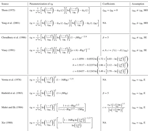
Table 1.Different parameterizations ofrHas compiled by Liu et al. (2007).

Source Parameterization ofrH Coefficients Assumption

Thom (1975) rH= 1 κ2_u

ln

_z−d z0m

−ψm(ζ ) ln _z−d

z0h

−ψh(ζ )

ζ0m=ζ0h=0 z0m6=z0h, MOST

Yang et al. (2001) rH= 1

κ2u

ln _z−d

z0m

−ψm(ζ, ζ0m) ln _z−d

z0h

−ψh(ζ, ζ0h)

NA z0m6=z0h, MOST

Choudhury et al. (1986) rH= 1

κ2u

ln _z−d

z0m ln

_z−d z0h

(1−βRiB)−3/4 β=5 z0m6=z0h, SE

Viney (1991) rH= 1 κ2_u

ln

_z−d z0m

ln _z−d

z0h

a+b(−RiB)c

−1

a, b, c=f ((z−d)/z0m) z0m6=z0h, SE

a=1.0591−0.0552 ln

1.72+h4.03−lnz_z−d 0m

i2

b=1.9117−0.2237 ln

1.86+h2.12−lnz_z−d 0m

i2

c=0.8437−0.1243 ln

3.49+h2.79−lnz_z−d 0m

i2

Verma et al. (1976) rH= 1

κ2u

ln _z−d

z0m 2

(1−16RiB)−1/4 NA z0m=z0h, E

Hatfield et al. (1983) rH= 1 κ2_u

ln

_z−d z0m

2

(1+βRiB) β=5 z0m=z0h, E

Mahrt and Ek (1984) rH= 1 κ2_u

ln

_z−d z0m

2" _1+c(−Ri B)1/2 1+c(−RiB)1/2−15RiB

#

c=

75κ2z−d+z0m

z_0m 1/2

h

lnz−d+z0m

z_0m

i2 z0m=z0h, E

Xie (1988) rH= 1 κ2_u

ln

_z−d z0m

2   1+

h

1−16RiBln _z−d

z0m i−1/2 lnz_z−d

0m

 

 NA z0m=z0h, E

(2007). These parameterizations based on MOST (Thom, 1975; Yang et al., 2001), empirical (E) (Verma et al., 1976; Hatfield et al., 1983; Mahrt and Ek, 1984; Xie, 1988) and semi-empirical (SE) (Choudhury et al., 1986; Viney, 1991) assumptions can be classified into two categories. Formula-tions by Thom (1975), Choudhury et al. (1986), Yang et al. (2001) and Viney (1991) have assumed z0m6=z0h, which should be a more realistic assumption. On the other hand, formulations by Verma et al. (1976), Hatfield et al. (1983), Mahrt and Ek (1984) and Xie (1988) assumed z0m=z0h. Different parameters used in the empirical formulations are also listed in Table 1.

One important point to note is that only the formulation by Yang et al. (2001) uses the stability parameters associated with the roughness lengthsζ0mandζ0h. Also note that all

pa-rameterizations assume a turbulent Prandtl number of unity; i.e., the diffusivities for momentum and heat are assumed to be the same. We shall later discuss the consequence of let-ting this parameter vary. Another important approximation necessary to evaluate all formulations in Table 1 is a pre-scription for the roughness lengthsz0m andz0h. Effects of different roughness lengths will be investigated in the fol-lowing section. However, a relation between the two rough-ness lengths (κB−1=ln(z0m/z0h)) was proposed by Owen and Thomson (1963) and Chamberlain (1968), whereκB−1 is called an “excess resistance parameter”. Yang et al. (2001) suggested an average value ofκB−1=2.0 (Liu et al., 2007), which will be used throughout this work.

8 and Table 1) is based on different variants of analytic ap-proximation approaches to reduce the complexity of flow in and above the forest canopy to a 2-D surface equivalent. It is widely accepted that the MOST approach is not completely accurate close to the canopy (Foken, 2006). It was proposed that a mixing length driven approach can be applied (Harman and Finnigan, 2007). Nonetheless, large-scale models, which cannot vertically resolve the canopies, still use MOST, and it has been demonstrated to be relatively accurate. Thus from an operational perspective, the present formulation revisits the current leading approach for simplification of the physics in a parameterized way that can be used by coarse-resolution models.

3 Methodology

The PALM large-eddy simulation model (Raasch and Schröter, 2001; Maronga et al., 2015) is used to investi-gate this generic nature of the canopy convector effect. The representation of the canopy in the LES follows the stan-dard distributed drag parameterization (Shaw and Schumann, 1992; Watanabe, 2004; Patton et al., 2015) by adding an ad-ditional term in the momentum budget equations as Fdi=

−Cda|u|ui, wherea is a one-sided frontal plant area

den-sity (PAD),Cd is a dimensionless drag coefficient assumed to be 0.3 (Katul et al., 2004; Banerjee et al., 2013), |u| is the wind speed, andui is the corresponding velocity

compo-nent (i=1,2,3, i.e.,u,v, andw). The effect of the canopy on the subgrid-scale (SGS) turbulence is accounted for by adding a sink term to the prognostic equation for the SGS turbulent kinetic energy (e) as F= −2Cda|u|e. For clo-sure of the SGS covariance terms, PALM uses the 1.5 or-der closure developed by Deardorff (1980) as modified by Moeng and Wyngaard (1988) and Saiki et al. (2000), which assumes a gradient-diffusion parameterization. The diffusiv-ities associated with this gradient diffusion are parameter-ized using the subgrid-scale turbulent kinetic energy (SGS-TKE) and include a prognostic equation for the SGS-TKE. This SGS-TKE scheme after Deardorff (1980) is deemed to be an improvement over the more traditional Smagorin-sky (1963) parameterization since the SGS-TKE allows for a much better estimation for the velocity scale correspond-ing to the subgrid-scale fluctuations (Maronga et al., 2015). Further details of the LES model can be found in the litera-ture and are not discussed here (Shaw and Schumann, 1992; Watanabe, 2004; Maronga et al., 2015; Patton et al., 2015). For our simulation, the number of grid points in thex,y, and z directions are 320, 320, and 640, respectively, with grid resolutions of 3.91, 3.91, and 1.95 m in the respective direc-tions. Each simulation has a simulated time of 10 000 s with a time step of 0.1 s, while the outputs of the first 6400 s are discarded before achieving computational quasi-equilibrium. The canopy height (hc) is taken as 35.0 m with a plant area index (PAI) of 5.0. It is important to note that Rotenberg

and Yakir (2011) reported an effective PAI of about 5–6 for heat exchange for the Yatir forest. This makes our PAI sim-ilar to a recent simulation study of Dias-Junior et al. (2015). In fact, as we already simulate a homogeneous canopy to show that the CCE appears more generically above vegeta-tion canopies, we have decided to tailor our simulavegeta-tions fol-lowing the examples of Patton et al. (2015) and Dias-Junior et al. (2015) in order to allow a better comparison of the LES data. The vertical distribution of plant area density (a) fol-lows the probability density function (pdf) of a Beta distribu-tion as described in Markkanen et al. (2003) and the param-etersαandβ controlling the vertical distribution of foliage are set as 3.0 and 2.0, respectively, to simulate a PAD dis-tribution similar to Dias-Junior et al. (2015). The parameters to drive the simulations for five different instability classes, namely, near neutral (NN), weakly unstable (WU), moder-ately unstable (MU), strongly unstable (SU), and free con-vection (FC), are similar to those of Patton et al. (2015) and are presented in Table 2. Note that the canopy convec-tor effect as a general phenomenon should not depend on water content in the soil–plant–atmosphere continuum and, moreover, the PALM-LES does not take into account any physiological processes which normally happen with a larger timescale. Nevertheless, instead of simulating a specific dry water free environment, some moisture at the lower surface is provided and the boundary conditions for surface moisture content are taken as similar to the simulations of Dias-Junior et al. (2015) as well. The initial conditions of the potential temperature (and moisture) profile are also taken as similar to Dias-Junior et al. (2015). PALM’s canopy module allows sensible heat flux input at the canopy top only, and the sen-sible heat flux is attenuated exponentially due to the decay of the incoming energy by absorption and reflection by the leaves. Thus the ground surface heat flux would be different from Patton et al. (2015). Another important point to note is that instead of lowering the wind speeds while maintaining similar sensible heat fluxes, the different stability classes can also be achieved by maintaining the same wind speed and ramping up the surface sensible heat fluxes. However, this should not affect the generic feature of the CCE as discussed at the end of Sect. 2.1. Further details and boundary condi-tions about the LES are discussed in Appendix B.

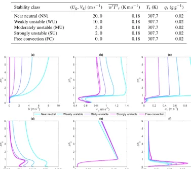
Table 2.Parameters to drive the simulations for five different instability classes, namely, near neutral (NN), weakly unstable (WU), mod-erately unstable (MU), strongly unstable (SU), and free convection (FC), are similar to Patton et al. (2015).UgandVgdenote geostrophic

wind speeds,w0_T0

tocdenotes canopy top surface sensible heat flux,Tsdenotes ground surface potential temperature, andqsdenotes specific

humidity at the ground surface.

Stability class (Ug,Vg) (m s−1) w0T0s(K m s−1) Ts(K) qs(g g−1)

Near neutral (NN) 20, 0 0.18 307.7 0.02 Weakly unstable (WU) 10, 0 0.18 307.7 0.02 Moderately unstable (MU) 5, 0 0.18 307.7 0.02 Strongly unstable (SU) 2, 0 0.18 307.7 0.02 Free convection (FC) 0, 0 0.18 307.7 0.02

Figure 1.Summary statistics of five LES simulations showing the variations between different stability classes in increasing order of insta-bility – from near neutral to free convection color coded as indicated in the legend.

4 Results and discussions 4.1 Comparison with LES

The results of the LES simulations are presented in Fig. 1 as temporally and spatially averaged vertical profiles for all five stability classes, where the lightest cyan shade indicates near neutral and the most magenta shade indicates free convec-tive conditions. Panel (a) shows the mean wind speed (U), panel (b) shows the standard deviation of longitudinal veloc-ity fluctuations (σu), and panel (c) shows the friction velocity

(which can be taken as a measure of turbulent intensity) (u∗) at every level for each simulation:

u∗=(u0_w02_+v0_w02₎1/4_{. (10)}

In the second row, panel (d) shows profiles of temporally and spatially averaged potential temperature (T), panel (e) shows the kinematic sensible heat flux (w0_T0_{), and panel (f) shows}

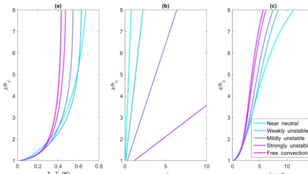
hori-Figure 2.Aerodynamic resistance to the heat transfer exhibiting the canopy convector effect.(a)Difference between surface and air temper-ature (Ts−Ta);(b)stability parameterζ;(c)canopy aerodynamic resistance (rH).

zontal velocity. For the same reasons, the turbulent intensity and friction velocity follow the same pattern. The strongly unstable cases have the highest heat fluxes, which is also physically consistent. Note that the canopy top sensible heat flux is similar to the imposed value of 0.18 K m s−1that was used to drive the simulations.

Figure 2 shows temporally and spatially averaged vertical profiles for the different stability conditions with the same color coding as Fig. 1. We investigate the vertical profile of rH in order to assess the uncertainty that arises from ing the reference height for the air temperature under vary-ing stability. The temperature of the canopy top is taken as the surface temperature (Ts) and thus results are shown from above the canopy top, i.e.,z/hc=1. Panel (a) shows the difference of surface and air temperature (Ts−Ta(z)). Panel (b) shows the stability parameterζ at every level com-puted asζ =(z−d)/Las explained in Sect. 2. Panel (c) plots canopy aerodynamic resistance to heat transfer (rH) at every level computed from Eq. (1). As is evident from panel (c), the aerodynamic resistance reduces with increasing instabil-ity, confirming the hypothesis constructed earlier and thus clearly demonstrating the canopy convector effect (CCE). As noted by Zilitinkevich et al. (2008), with increasing in-stability, “convective updraughts developing at side walls of roughness elements extend upwards and provide extra re-sistances to the mean flow. Then the mean flow interacts with both solid obstacles and their virtual extensions (up-draughts), which results in the increased roughness length”. This increased roughness can be recognized as the aerody-namic roughness. For the same physical roughness of the canopy, an increase in instability increases this aerodynamic roughness and, in turn, reducesrH. The low aerodynamic re-sistance effectively allows larger eddies to form above the forest canopy which are more efficient to dissipate the sen-sible heat by promoting buoyancy. This description refers to a more general phenomenon as opposed to the description

by Rotenberg and Yakir (2011) which identifies the higher physical roughness of the canopy compared to the desert and is thus a more site specific description. Nevertheless, it is ac-knowledged that the more generic description presented here can be reconciled with the explanation from Rotenberg and Yakir (2011) by noting that increased physical roughness can also result in increased aerodynamic roughness. Also inci-dentally, RY10 reported a value ofrH≈16 for the Yatir for-est which is of similar order of magnitude as what is found in panel (c) of Fig. 2. One important point to note in Fig. 1 is the magnitude of the Prandtl number, which is almost fixed to about 0.335 above the canopy. This can be reconciled with the theoretical prediction of the variation ofPr0with stability by Li et al. (2015). For stability ranges 1≤ −ζ ≤10,Pr0is also estimated to be approximately 0.33, consistent with the stability ranges plotted in Fig. 2. The variation ofPr0 with stability is discussed further in Appendix A.

4.2 Testing different parameterizations

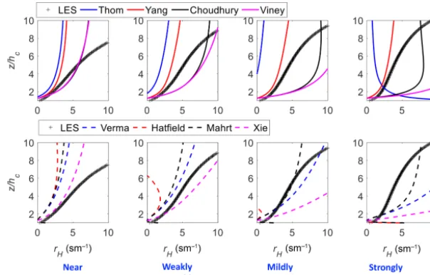
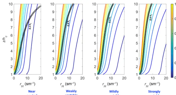
Figure 3.Variations ofrH with height across stability ranges and comparisons with different parameterization schemes as described in

Table 1.

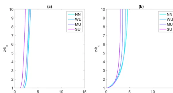
Figure 4.Variations ofrHwith height for different stability classes computed for each parameterization scheme as described in Table 1.

et al. (1976) (blue dashed line), Hatfield et al. (1983) (red dashed line), Mahrt and Ek (1984) (black dashed line), and Xie (1988) (pink dashed line). It should be noted that a single value of roughnessz0m=0.6hchas been chosen for all cases by trial and error to obtain a “good” comparison in Fig. 3. As observed, none of the parameterizations can capture the cor-rect height variations of rH, except the one by Yang et al. (2001) for more unstable cases. However, all parameteriza-tions seem to do a decent job close to the canopy top. This clearly indicates that one single value forz0mas suggested by these parameterizations is inadequate. To study whether the different parameterization schemes can capture the canopy convector effect, rH computed from each method is plot-ted for different heights for the different stability classes in Fig. 4. The title of each panel describes which parameter-ization is plotted and the color shades starting from cyan to purple indicate increasing instability. As is evident, only

the parameterization by Thom (1975) captures the canopy convector effect for weaker instabilities. The parameteriza-tion by Yang et al. (2001) also displays the signatures of the CCE, however weakly. The other formulations cannot cap-ture the correct trend of the CCE at all. Thus at this stage it is clear that the Yang et al. (2001) formulation, based on MOST and distinguishing between two different roughness lengths, is the most promising candidate for parameterizingrH com-pared to the other formulations which apply some form of approximation or do not apply MOST.

com-Figure 5.Variations ofrHas given by the parameterization of Yang et al. (2001) with height across stability ranges and a wide range ofz0m.

Black “+” markers indicate the observedrHfrom LES at any particular stability state.

puted across a wide range ofz0mand compared with the LES outputs for the different stability classes. As observed, an in-crease inz0mwith increasing instability captures the height variation better than a single roughness length for all stability classes, further providing support for the notion put forward by Zilitinkevich et al. (2008). Hence the formulation by Yang et al. (2001) can be modified to include the effects of stratifi-cation on several parameters. Zilitinkevich et al. (2008) sug-gested a stability dependent zero-plane displacement length as well as a stability dependent z0m based on dimensional analysis, given by

ds=

d

1+0.56hc −L

1/3,

(11)

and z0ms=z0m

"

1+1.15

_h

c −L

1/3#

, (12)

wheredsandz0msare the stability dependent zero-plane dis-placement length and roughness lengths for momentum, re-spectively, d andz0m being their neutral counterparts.d= (2/3)hccan be assumed as usual. The neutralz0mcan be as-sumed to be related to LAI as given by Shuttleworth and Gur-ney (1990). According to the relation used by Shuttleworth and Gurney (1990), for an LAI of 5,z0m=0.12hccan be ob-tained (which is almost constant for a wide range of canopy drag coefficients and LAI). Moreover, if one uses the correct stability dependent Prandtl numberPr0(ζ )instead of setting it to unity, an improved parameterization based on Yang et al. (2001) can be written as

rH=

Pr0(ζ ) κ2_u

ln

_z−d s z0ms

−ψm(ζ, ζ0ms)

ln

z−ds

z0hs

−ψh(ζ, ζ0hs)

. (13)

Figure 6. (a)The variation ofrHwith height across stability according to the improved formulation as given by Eq. (13);(b)similar variations

ofrHcomputed from the LES repeated again for comparison.

Figure 7. (a)The variation ofrHwith height across stability according to the improved formulation as modeled by Eq. (13), but using the

top-of-canopy surface flux throughout all heights;(b)similar variations ofrHcomputed from the LES using the top-of-canopy surface flux

assumed to be constant in the surface layer.

5 Conclusion

The canopy aerodynamic resistance is a concept borrowed from the evapotranspiration literature where it represents the resistance between the idealized “big-leaf” (a reduced-order representation of the fully heterogeneous 3-D canopy) and the atmosphere for heat or vapor transfer (Alves et al., 1998). In semi-arid ecosystems, vegetation canopies maintain a rel-atively cool surface temperature in spite of the high sensible heat flux by reducing the canopy aerodynamic resistance to heat transfer (rH) – a phenomenon named the “canopy con-vector effect” by Rotenberg and Yakir (2010). In the present work, a large-eddy simulation is used to examine this canopy convector effect and, in the process, several existing param-eterizations forrH are examined. The objectives behind this exploration are 2-fold. The first one is to investigate whether the existing parameterizations exhibit the canopy convector

de-scribe the correct trend of the CCE. Among different formu-lations, the one by Yang et al. (2001) is found to be the most promising candidate. This parameterization employs MOST, and accounts for stability parameters associated with rough-ness lengths for momentum and heat transfer. It is found that a stability dependent zero-plane displacement height as well as stability dependent roughness lengths for momentum and heat transfer can improve its performance. Moreover, if the surface layer or the canopy sublayer is assumed to have a constant sensible heat flux equal to the flux at the canopy top, and a stability dependent Prandtl number is used, the performance improves further. These assumptions also lead to a less nonlinear height variation. These explorations high-light the uncertainties associated with the parameterizations of rH. One possible major source of uncertainty is the us-age of Monin–Obukhov similarity theory in the canopy sub-layer (CSL) (up to 3hcto 6hc) since it is not expected to per-form in the CSL (Kaimal and Finnigan, 1994). Nevertheless,

MOST formulations are found to outperform other semi-empirical formulations using Richardson numbers. Thus fu-ture research work will involve studying these uncertainties ofrHparameterizations in regional and global climate mod-els. The consequence of this CCE for local circulation, at-mospheric moisture, and tree physiology will also be investi-gated, extending the preliminary study of Eder et al. (2015). However, the fact that the CCE is a more generic feature of canopy turbulence provides hope that the afforestation of an area larger than the Yatir forest would also be able to cope with a high-radiation load under water scarcity in semi-arid climates.

Appendix A: Stability dependence of the Prandtl number

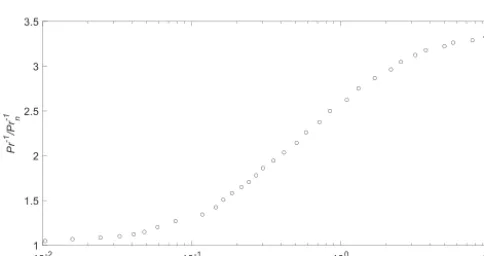
The turbulent Prandtl numberPr0is defined as the ratio of the eddy diffusivities of momentum and heat (Km/Kh). The variation of the Prandtl number with stability (Pr0(ζ )) was discussed in detail by Li et al. (2015) by using a spectral bud-get formulation and is not repeated here. Only the predicted variation ofPr−1/Pr−_n1with stability (ζ =z/L) is digitized and produced in Fig. A1, which was experimentally validated by Li et al. (2015). Pr−_n1denotes the inverse of the neutral Prandtl number which can assumed to be equal to 1. Note that for the stability ranges computed in the LES simulations in Fig. 2, this formulation predicts a Pr0≈0.33, which is also observed in thePr0independently computed in Fig. 1.

Figure A1.The variation ofPr−1/Pr−n1with stability according to

the spectral budget formulation of Li et al. (2015).

Appendix B: Some computational details of the LES B1 Surface heat flux formulation and

boundary conditions

The ground surface heat flux for grid points with a canopy layer is given by

w0_T0

s=w0T0toc×exp 

−c

hc Z

0

LAD(z)dz 

, (B1)

withc=0.6 the extinction coefficient of light within the canopy. Within the canopy the plant-canopy heating rate is calculated as the vertical divergence of the canopy heat fluxes:

w0_T0 toc

d dzexp



c

hc Z

z

LAD(z0)dz0 

. (B2)

The bottom boundary condition for potential temperature is a Neumann condition; the boundary condition at the top of the domain is such that the initial temperature gradient is maintained at the top of the domain.

B2 Eddy diffusivity formulation

The computation for the eddy diffusivities in PALM follows the standard procedure for 1.5 order turbulence closure. Thus they are computed from the subgrid-scale turbulent kinetic energy, more precisely Eqs. (13)–(14) from Maronga et al. (2015).

Eddy diffusivity for momentum: Km=cml

√

e. (B3)

Eddy diffusivity for heat: Kh=

1+2l

1

Km, (B4)

Author contributions. TB conceived the idea, conducted data anal-ysis, and wrote the paper. FDR set up the large-eddy simulations. MM had written the proposal that funded this project, supervised the project, and provided comments and suggestions.

Competing interests. The authors declare that they have no conflict of interest.

Acknowledgements. This research was supported by the German Research Foundation (DFG) as part of the “Climate feedbacks and benefits of semi-arid forests (CliFF)” project and the “Capturing all relevant scales of biosphere–atmosphere exchange – the enigmatic energy balance closure problem” project, which are funded by the Helmholtz Association through the President’s Initiative and Networking Fund, and by the KIT. The authors thank the PALM group at Leibniz University Hannover for their open-source PALM code and also thank Dan Yakir and Eyal Rotenberg at the Weizmann Institute of Science, Israel, for their support during the CliFF campaign. We thank Thomas Foken, Bayreuth center of Ecology and environmental Research (BayCEER), University of Bayreuth, Germany, for his comments and suggestions. We also thank Gil Bohrer, (Ohio State University) and the other, anonymous, reviewer for their constructive suggestions to improve the manuscript during the discussion stage.

The service charges for this open access publication have been covered by a Research Centre of the Helmholtz Association.

Edited by: Pierre Gentine

Reviewed by: Gil Bohrer and one anonymous referee

References

Allen, R. G., Pereira, L. S., Raes, D., and Smith, M.: Crop evapotranspiration-Guidelines for computing crop water requirements-FAO Irrigation and drainage paper 56, FAO, Rome: Food and Agriculture Organization of the United Nations, 300, 1998.

Alves, I., Perrier, A., and Pereira, L.: Aerodynamic and surface re-sistances of complete cover crops: How good is the “big leaf”?, T. ASAE, 41, 345–352, 1998.

Baldocchi, D., Falge, E., Gu, L., Olson, R., Hollinger, D., Running, S., Anthoni, P., Bernhofer, C., Davis, K., Evans, R., Fuentes, J., Goldstein, A., Katul, G., Law, B., Lee, X., Malhi, Y., Meyers, T., Munger, W., Oechel, W., Paw U, K. T., Pilegaard, K., Schmid, H. P., Valentini, R., Verma, S., Vesala, T,. Wilson, K., and Wofsy, S.: FLUXNET: a new tool to study the temporal and spatial variabil-ity of ecosystem-scale carbon dioxide, water vapor, and energy flux densities, B. Am. Meteorol. Soc., 82, 2415–2434, 2001. Banerjee, T., Katul, G., Fontan, S., Poggi, D., and Kumar, M.:

Mean flow near edges and within cavities situated inside dense canopies, Bound.-Lay. Meteorol., 149, 19–41, 2013.

Chamberlain, A.: Transport of gases to and from surfaces with bluff and wave-like roughness elements, Q. J. Roy. Meteor. Soc., 94, 318–332, 1968.

Choudhury, B., Reginato, R., and Idso, S.: An analysis of infrared temperature observations over wheat and calculation of latent heat flux, Agr. Forest Meteorol., 37, 75–88, 1986.

Cleverly, J., Chen, C., Boulain, N., Villalobos-Vega, R., Faux, R., Grant, N., Yu, Q., and Eamus, D.: Aerodynamic resistance and Penman-Monteith evapotranspiration over a seasonally two-layered canopy in semiarid central Australia, J. Hydrometeorol., 14, 1562–1570, 2013.

Deardorff, J. W.: Stratocumulus-capped mixed layers derived from a three-dimensional model, Bound.-Lay. Meteorol., 18, 495–527, 1980.

Dias-Junior, C. Q., Marques Filho, E. P., and Sá, L. D.: A large eddy simulation model applied to analyze the turbulent flow above Amazon forest, J. Wind Eng. Ind. Aerodyn., 147, 143–153, 2015. Dyer, A.: A review of flux-profile relationships, Bound.-Lay.

Mete-orol., 7, 363–372, 1974.

Dyer, A. and Hicks, B.: Flux-gradient relationships in the constant flux layer, Q. J. Roy. Meteor. Soc., 96, 715–721, 1970.

Eder, F., De Roo, F., Rotenberg, E., Yakir, D., Schmid, H. P., and Mauder, M.: Secondary circulations at a solitary forest surrounded by semi-arid shrubland and their impact on eddy-covariance measurements, Agr. Forest Metereol., 211, 115–127, 2015.

Foken, T.: 50 years of the Monin-Obukhov similarity theory, Bound.-Lay. Meteorol., 119, 431–447, 2006.

Foken, T., Dlugi, R., and Kramm, G.: On the determination of dry deposition and emission of gaseous compounds at the biosphere-atmosphere interface, Meteorol. Z, 4, 91–118, 1995.

Garratt, J. R.: Aerodynamic roughness and mean monthly surface stress over Australia, 29, Commonwealth Scientific and Indus-trial Research Organization, Melbourne, 1977.

Harman, I. N. and Finnigan, J. J.: A simple unified theory for flow in the canopy and roughness sublayer, Bound.-Lay. Meteorol., 123, 339–363, 2007.

Hatfield, J., Perrier, A., and Jackson, R.: Estimation of evapotran-spiration at one time-of-day using remotely sensed surface tem-peratures, Agr. Water. Manage., 7, 341–350, 1983.

Kaimal, J. C. and Finnigan, J. J.: Atmospheric boundary layer flows: their structure and measurement, Oxford University Press, 1994. Katul, G. G., Mahrt, L., Poggi, D., and Sanz, C.: One-and two-equation models for canopy turbulence, Bound.-Lay. Meteorol., 113, 81–109, 2004.

Li, D., Katul, G. G., and Zilitinkevich, S. S.: Revisiting the turbu-lent Prandtl number in an idealized atmospheric surface layer, J. Atmos. Sci., 72, 2394–2410, 2015.

Liu, S., Lu, L., Mao, D., and Jia, L.: Evaluating parame-terizations of aerodynamic resistance to heat transfer using field measurements, Hydrol. Earth Syst. Sci., 11, 769–783, https://doi.org/10.5194/hess-11-769-2007, 2007.

Mahrt, L. and Ek, M.: The influence of atmospheric stability on po-tential evaporation, J. Clim. Appl. Meteorol., 23, 222–234, 1984. Markkanen, T., Rannik, Ü., Marcolla, B., Cescatti, A., and Vesala, T.: Footprints and fetches for fluxes over forest canopies with varying structure and density, Bound.-Lay. Meteorol., 106, 437– 459, 2003.

formulation, recent developments, and future perspectives, Geosci. Model Dev., 8, 2515–2551, https://doi.org/10.5194/gmd-8-2515-2015, 2015.

Maurer, K. D., Bohrer, G., Kenny, W. T., and Ivanov, V. Y.: Large-eddy simulations of surface roughness parameter sensitivity to canopy-structure characteristics, Biogeosciences, 12, 2533– 2548, https://doi.org/10.5194/bg-12-2533-2015, 2015.

Maurer, K. D., Hardiman, B. S., Vogel, C. S., and Bohrer, G.: Canopy-structure effects on surface roughness parameters: Ob-servations in a Great Lakes mixed-deciduous forest, Agr. Forest Meteorol., 177, 24–34, 2013.

Moeng, C.-H. and Wyngaard, J. C.: Spectral analysis of large-eddy simulations of the convective boundary layer, J. Atmos. Sci., 45, 3573–3587, 1988.

Monteith, J.: Principles of environmental physics, Academic Press, London, England, 1973.

Monteith, J. and Unsworth, M.: Principles of Environmental Physics, Academic Press, London, England, 2007.

Owen, P. and Thomson, W.: Heat transfer across rough surfaces, J. Fluid Mech., 15, 321–334, 1963.

Patton, E. G., Sullivan, P. P., Shaw, R. H., Finnigan, J. J., and Weil, J. C.: Atmospheric stability influences on coupled boundary-layer-canopy turbulence, J. Atmos. Sci., 73, 1621–1648, 2015. Paulson, C. A.: The mathematical representation of wind speed and

temperature profiles in the unstable atmospheric surface layer, J. Appl. Meteorol., 9, 857–861, 1970.

Penman, H. L.: Natural evaporation from open water, bare soil and grass, P. Roy. Soc. Lond. A, 193, 120–145, 1948.

Raasch, S. and Schröter, M.: PALM–a large-eddy simulation model performing on massively parallel computers, Meteorol. Z., 10, 363–372, https://doi.org/10.1127/0941-2948/2001/0010-0363, 2001.

Rotenberg, E. and Yakir, D.: Contribution of semi-arid forests to the climate system, Science, 327, 451–454, 2010.

Rotenberg, E. and Yakir, D.: Distinct patterns of changes in surface energy budget associated with forestation in the semiarid region, Glob. Change Biol., 17, 1536–1548, 2011.

Saiki, E. M., Moeng, C.-H., and Sullivan, P. P.: Large-eddy simula-tion of the stably stratified planetary boundary layer, Bound.-Lay. Meteor., 95, 1–30, 2000.

Seginer, I.: Aerodynamic roughness of vegetated surfaces, Bound.-Lay. Meteorol., 5, 383–393, 1974.

Shaw, R. H. and Schumann, U.: Large-eddy simulation of turbulent flow above and within a forest, Bound.-Lay. Meteorol., 61, 47– 64, 1992.

Shuttleworth, W. J. and Gurney, R. J.: The theoretical relation-ship between foliage temperature and canopy resistance in sparse crops, Q. J. Roy. Meteorol. Soc., 116, 497–519, 1990.

Smagorinsky, J.: General circulation experiments with the primitive equations: I. the basic experiment, Mon. Weather Rev., 91, 99– 164, 1963.

Stull, R. B.: An introduction to boundary layer meteorology, Vol. 13, Springer Science & Business Media, 2012.

Thom, A.: Momentum, mass and heat exchange of plant communi-ties, Vol. 1, Academic Press, London, 1975.

Verma, S., Rosenberg, N., Blad, B., and Baradas, M.: Resistance-energy balance method for predicting evapotranspiration: Deter-mination of boundary layer resistance and evaluation of error ef-fects, Agron. J., 68, 776–782, 1976.

Viney, N. R.: An empirical expression for aerodynamic resistance in the unstable boundary layer, Bound.-Lay. Meteorol., 56, 381– 393, 1991.

Walko, R. L., Band, L. E., Baron, J., Kittel, T. G., Lammers, R., Lee, T. J., Ojima, D., Pielke Sr., R. A., Taylor, C., Tague, C., Trem-back, C. J., and Vidale, P. L.: Coupled atmosphere-biophysics-hydrology models for environmental modeling, J. Appl. Meteo-rol., 39, 931–944, 2000.

Watanabe, T.: Large-eddy simulation of coherent turbulence struc-tures associated with scalar ramps over plant canopies, Bound.-Lay. Meteorol., 112, 307–341, 2004.

Webb, E.: On the correction of flux measurements for effects of heat and water vapour transfer, Bound.-Lay. Meteorol., 23, 251–254, 1982.

Xie, X.: An improved energy balance-aerodynamic resistance model used estimation of evapotranspiration on the wheat field, Acta Meteorol. Sin., 46, 102–106, 1988 (in Chinese).

Yang, K., Tamai, N., and Koike, T.: Analytical solution of surface layer similarity equations, J. Appl. Meteorol., 40, 1647–1653, 2001.