www.hydrol-earth-syst-sci.net/21/2233/2017/ doi:10.5194/hess-21-2233-2017
© Author(s) 2017. CC Attribution 3.0 License.
Historical and future trends in wetting and drying
in 291 catchments across China
Zhongwang Chen1,2, Huimin Lei1,2, Hanbo Yang1,2, Dawen Yang1,2, and Yongqiang Cao3 1Department of Hydraulic Engineering, Tsinghua University, Beijing, 100084, China
2State Key Laboratory of Hydro-Science and Engineering, Tsinghua University, Beijing, 100084, China 3School of Urban Planning and Environmental Science, Liaoning Normal University, Dalian, 116029, China
Correspondence to:Hanbo Yang ([email protected]) Received: 11 November 2016 – Discussion started: 25 November 2016
Revised: 9 March 2017 – Accepted: 27 March 2017 – Published: 26 April 2017
Abstract. An increasingly uneven distribution of hydrome-teorological factors related to climate change has been de-tected by global climate models (GCMs) in which the pat-tern of changes in water availability is commonly described by the phrase “dry gets drier, wet gets wetter” (DDWW). However, the DDWW pattern is dominated by oceanic ar-eas; recent studies based on both observed and modelled data have failed to verify the DDWW pattern on land. This study confirms the existence of a new DDWW pattern in China after analysing the observed streamflow data from 291 Chi-nese catchments from 1956 to 2000, which reveal that the distribution of water resources has become increasingly un-even since the 1950s. This pattern can be more accurately described as “drier regions are more likely to become drier, whereas wetter regions are more likely to become wetter”. Based on a framework derived from the Budyko hypothesis, this study estimates runoff trends via observations of precipi-tation (P) and potential evapotranspiration (Ep) and predicts the future trends from 2001 to 2050 according to the projec-tions of five GCMs from the Coupled Model Intercompari-son Project Phase 5 (CMIP5) under three scenarios: RCP2.6, RCP4.5, and RCP8.5. The results show that this framework has a good performance for estimating runoff trends; such changes in P play the most significant role. Most areas of China, including more than 60 % of catchments, will expe-rience water resource shortages under the projected climate changes. Despite the differences among the predicted results of the different models, the DDWW pattern does not hold in the projections regardless of the model used. Nevertheless, this conclusion remains tentative owing to the large uncer-tainties in the GCM outputs.
1 Introduction
Terrestrial water availability is critical to human lives and economic activities (Milly et al., 2005). In recent decades, changes in water availability have had significant effects on human society (Piao et al., 2010) and the environment (Ar-nell, 1999) in the context of climate change. Runoff (Q) is a commonly adopted indicator of water availability (Milly et al., 2005). The response of Q to climate change has been widely investigated from basin scale to global scales based on streamflow observations (e.g. Pasquini and De-petris, 2007; Dai et al., 2009; Stahl et al., 2010) or model outputs (e.g. Hamlet et al., 2007; Alkama et al., 2013; Greve et al., 2014).
ex-ploring whether a similar effect in Qexists on land as the “dry gets drier, wet gets wetter” (DDWW) pattern found in P −E, which indicates increasingly uneven distribution of the water resources. The original DDWW pattern predicted a simple active proportional relationship betweenP−Eand 1(P−E), where the sign of P−E determines whether a region is dry (negative) or wet (positive). It should be noted that the predicted changes are averages of latitudinal zones rather than values at the local scale (e.g. grid box or catch-ment). This results in dominance of the oceanic components in the DDWW pattern (Roderick et al., 2014) because P andE are dominated by exchanges over the ocean at most latitudes (Lim and Roderick, 2009). Thus, the DDWW pat-tern is more appropriately applied to oceans than to land. In fact, because the long-term mean P−E is overwhelm-ingly positive on land, the method of using the sign ofP−E to identify wet and dry regions is no longer feasible be-cause1(P−E)can obviously be negative. Therefore, some scholars attempted to explore a new DDWW pattern to de-scribe changes in the hydrological cycle on land at the lo-cal slo-cale. Greve et al. (2014) adopted the aridity index (ϕ
=Ep/P, whereEpdenotes the potential evapotranspiration) to measure the aridity degree and defined ϕ >2 as dry re-gions andϕ <2 as wet regions. Consequently, the pattern be-cameϕ >2,1(P−E) <0, whereasϕ <2,1(P−E) >0. However, the results, based on more than 300 combinations of various global hydrological data sets containing both ob-served and modelled data, showed that only 10.8 % of land areas robustly followed the adjusted DDWW pattern. Never-theless, the study of Greve et al. (2014) still has some defects related to two major aspects. The first is the existence of large uncertainties in E in both satellite-based observations and simulations (Kumar et al., 2016), and the second is the arti-ficially assigned threshold between the wet and dry regions, which likely leads to different results when the threshold is changed. Therefore, a study based on observedQdata that are more direct and of relatively low uncertainty should be conducted, and a new method should be adopted to partition dry and wet regions independent of the appointed threshold. However, it should be noted that the observed changes in Qare responses not only to climate change but also to other factors such as land cover changes and human activ-ities, e.g. withdrawal and drainage (Stahl et al., 2010). To extract the components related only to climate change is an intractable process because no effective method has been pre-sented thus far. Therefore, a roundabout means is to com-pare credibly estimated changes inQunder climate change with the estimate based on observed data. The Budyko hy-pothesis (Budyko, 1948) is an effective and simple tool for modelling the mean annualQwithin a catchment based only on meteorological information (Koster and Suarez, 1999). The Budyko hypothesis depicts the long-term coupled water-energy balance for a catchment as
E/P=f Ep/P , c, (1)
where the functionf denotes Budyko-like equations,Epis the mean annual potential evapotranspiration, and c is a parameter characterizing a particular catchment. There are various types of Budyko-like equations (e.g. Pike, 1964; Fu, 1981; Choudhury, 1999; Zhang et al., 2001; Yang et al., 2008; Wang and Tang, 2014; Zhou et al., 2015). The Budyko hypothesis has been examined and applied in both observation-based (Zhang et al., 2001; Oudin et al., 2008; Xu et al., 2014) and model-based studies (Zhang et al., 2008; Teng et al., 2012), producing good consistency between ob-served and modelled data. By analysing hydrometeorologi-cal data from 108 non-humid catchments in China, Yang et al. (2007) confirmed that the Budyko hypothesis is capable of predictingQboth at long-term and annual timescales. Xiong and Guo (2012) assessed the Budyko hypothesis in 29 hu-mid watersheds in southern China and found that parametric Budyko formulae can effectively estimate the long-term av-erageQ. Therefore, it is reasonable to estimateQby using the Budyko hypothesis in China. The ability of the Budyko hypothesis to capture the effects of climate change onQ, as well as other details, is described in Sect. 2.3.
Based on observed streamflow data from 291 catchments in China, this study first analyses the historical trends in an-nualQto explore the possible existence of a DDWW pat-tern via a new method proposed in Sect. 2.2. Then, by adopt-ing a simple framework derived from the Budyko hypothe-sis stated in Sect. 2.3, this study estimates the runoff trends caused by climate change in the study catchments to re-veal that the historical trends are mainly a response to cli-mate change and to identify the key influencing factor. More-over, based on the Coupled Model Intercomparison Project Phase 5 (CMIP5) projections of five GCMs, this study pre-dicts changes inQvia the framework to determine whether the DDWW pattern will continue to hold in the future.
2 Data and methods 2.1 Study area and data
con-130° E 120° E
110° E 100° E
90° E 80° E
70° E 50° N
40° N
30° N
20° N
River basin
First level watershed boundary Southeast Rivers Inland River Songhua River Hai He River
[image:3.612.126.467.69.289.2]Pearl River Southwest River Liao River Yangtze River Yellow River
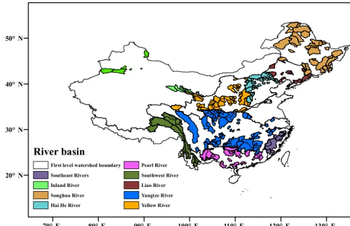
Figure 1.Spatial distribution of the 291 study catchments across mainland China.
sumption and removing the supplement. The water consump-tion includes the net consumpconsump-tion in agricultural, industrial, and residential sectors as well as water loss in the reservoir owing to evaporation and leakage. The water supplement includes the water diverted from other watersheds and the part of the extracted groundwater supplied back to the river. Changes in the reservoir storage can depend on whether the change is positive or negative. Thus, the restored discharge can be considered as the approximate natural discharge. The records range in length from 21 to 45 years; 261 catchments have record lengths greater than 40 years.
Two meteorological data sets were used in this study. The first is the 10 km gridded data set interpolated by Yang et al. (2014) based on 736 stations of the China Meteo-rological Administration, which includes P and potential evapotranspiration (Ep) observations from 1956 to 2000. Based on this observed data set, the annual arealP andEp of each catchment were calculated. The other is the daily bias-corrected (Piani et al., 2010; Hagemann et al., 2011) modelled data set from the Inter-Sectoral Impact Model Intercomparison Project (ISI-MIP; http://www.isi-mip.org) covering the period 1951–2050 under scenarios RCP2.6, RCP4.5, and RCP8.5, as released by the CMIP5. The mod-elled data were initially downscaled to a 0.5◦×0.5◦latitude– longitude grid data set and were then extracted and trans-formed into the ASCII format by the Institute of Environ-ment and Sustainable DevelopEnviron-ment in Agriculture, Chinese Academy of Agricultural Sciences, China. The output data for each scenario include precipitation; mean, maximum, and minimum air temperature; solar radiation; wind speed; and relative humidity for the five models including GFDL-ESM2M, HadGEM2-ES, IPSL-CM5A-LR,
MIROC-ESM-CHEM, and NorESM1-M. The daily Ep of each grid was estimated by adopting the Penman equation (Penman, 1948; Appendix A) based on the GCM outputs. The annual series ofP andEpwere calculated as the sum of every dailyP and Ep over one year. Then, the annual catchment-averagedP andEpwere calculated as the average of griddedP andEp within one catchment.
2.2 Runoff trends and DDWW pattern
In this study, two slightly different methods were used to esti-mate the runoff trend for the historical (1956–2000) and pro-jected periods (2001–2050), respectively. The runoff trend for the historical period was estimated as the slope of the lin-ear regression of the annualQseries, denoted askQ, and can
be calculated by
kQ= m P i=1
ti−t Qi−Q
m P i=1
ti−t2
, (2)
wheremis the observed record length of a catchment, iis theith record,ti is the year of this record,t is the average
of all recorded years, andQi andQare the observed annual
runoff inti and the mean annual runoff in the historical
pe-riod, respectively. The significance ofkQwas tested by using
at test. The runoff trend of the projected period, denoted as 1Q, is defined as the change in mean annual runoff between historical and projected periods and can be computed as
1Q=Qp−Q, (3)
130° E 120° E 110° E 100° E 90° E 80° E 70° E 50° N
40° N
30° N
20° N
10° N
130° E 120° E 110° E 100° E 90° E 80° E 70° E 50° N
40° N
30° N
20° N
10° N
Mean annual runoff (mm)
0 200 400 600 800 1000 1200 1400
Aridity index
0.5 2/3 1 1.5 2 3 8
[image:4.612.102.496.69.208.2](a)
(b)
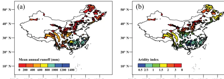
Figure 2.Spatial distribution of(a)mean annual runoff and(b)aridity indexϕin the 291 study catchments.
In the study of Greve et al. (2014), the DDWW pattern was sensitive to the assigned threshold for defining the dry and wet regions such that different thresholds may have led to different, and possibly conflicting, results. To remove the influence of the threshold, Allan et al. (2010) adopted per-centile bins for P to define wet and dry regions, thereby successfully avoiding the pitfalls of selecting a convincing threshold. Therefore, this study does not define absolute wet or dry regions but instead identifies relatively wetter or drier ones. Specifically, two variables, Qandϕ, were chosen as indicators of the aridity degree. The termϕ was introduced to maintain consistency with studies based on the climate model data where Q is not available. The spatial distribu-tions ofQandϕ are shown in Fig. 2, withQranging from 0 to 1400 mm a−1andϕ ranging from 0.5 to 8. We divided Q andϕ into six intervals, where the intervals with larger Q values and smaller ϕ values denoted wetter levels (Ta-ble 1). In each interval, the total catchments and catchments becoming wetter were counted, and then the proportion of catchments becoming wetter, denoted asd, was calculated. A largerd value implies that more catchments have become wetter in this level. This study compares thedvalues of dif-ferent intervals to examine a new DDWW pattern.
2.3 Framework for estimating runoff trends under climate change
Among various types of Budyko-like equations, two analyt-ical equations proposed by Fu (1981) and Yang et al. (2008) should be highlighted. These two equations are able to bet-ter capture the role of landscape characbet-teristics because the two studies each introduce a catchment property parameter, ωandn, respectively, as shown by the two examples ofcin Eq. (1). Yang et al. (2008) showed a high linear correlation betweenωandn. Therefore, this study adopted the equation derived by Yang et al. (2008), which has been rewritten as
Table 1.Details of the interval partitions based on observed mean annual runoffQand aridity indexϕ.
Interval Interval Sample
number range size
Based onQ
1 0–200 141
2 200–400 42
3 400–600 31
4 600–800 26
5 800–1000 32
6 1000–1400 19
Based onϕ
1 0.5–2/3 21
2 2/3–1 72
3 1–1.5 33
4 1.5–2 55
5 2–3 68
6 3–8 42
E
P
=
" Ep
P !−n
+1
#−1/n
. (4)
Focusing onQ, this study transformed Eq. (4) into
Q=P−P "
Ep P
!−n
+1
#−1/n
. (5)
The parameterncan be calculated by using the observedQ, P, andEp of each catchment from the period 1956–2000. The differential form of Eq. (5) was derived as
dQ=∂Q
∂PdP+ ∂Q ∂Ep
dEp+ ∂Q
∂ndn, (6)
[image:4.612.311.543.278.624.2]mean values. Equation (6) has widely been used to estimate changes in annual Q(e.g. Yang and Yang, 2011; Roderick and Farquhar, 2011; Roderick et al., 2014).
Because we focused on the effects of climate change, n was assumed to remain unchanged, i.e. dn=0 (Yang and Yang, 2011), and Eq. (6) became
dQ=∂Q
∂PdP+ ∂Q ∂Ep
dEp. (7)
For convenience, we introducedεP andε0to represent ∂Q∂P and ∂E∂Q
p, which can be estimated on the basis ofn,P, and
Ep:
εP = ∂Q ∂P
P ,Ep
=1−
"
1+ Ep
P
!−n#−n
+1
n
and
ε0= ∂Q ∂Ep
P ,Ep
= −
"
1+ Ep
P
!n#−n+n1
.
Roderick et al. (2014) showed that the runoff changes (=1(P−E)in this study) estimated by using Eq. (7) ac-count for about 82 % of the variation in the GCM projections of 1(P−E). Therefore, Eq. (7) can predict a reliable re-sult under climate change projected by the GCMs. Based on Eq. (7), a framework can then be constructed to estimate the runoff trends and is interpreted in Appendix B:
kQe=εPkP+ε0kEp, (8a)
1Qe=εP1P+ε01Ep, (8b)
wherekQe and1Qe are estimated runoff trends of the his-torical and projected periods, respectively; kP andkEp are
the linear regression-calculated trends in annual P andEp, respectively; and 1P and1Ep are changes in P andEp, respectively.
Equation (8a) and (8b) attribute the runoff trend to two major factors: the precipitation trend and the potential evapo-transpiration trend. Equation (8a) estimateskQeaccording to
the observedkP andkEp. Equation (8b) estimates1Qe ac-cording to the GCM projections, where1P and1Epare cal-culated as the differences inP andEpbetween 1956–2000 and 2001–2050. To measure the uncertainty of the GCMs, the coefficient of variance (Cv) in each catchment was estimated. Cvis defined as the ratio between the standard deviation and the absolute mean of the five1Qeoutputs of the respective GCMs. Specifically, a lowerCvindicates less uncertainty in 1Qebecause the results of the different GCMs are similar.
130° E 120° E
110° E 100° E
90° E 80° E
50° N
40° N
30° N
20° N Significant catchments
[image:5.612.308.545.66.219.2] [image:5.612.45.228.238.335.2]< -6 -4 -2 0 2 4 6 8 < (mm a-1)
Figure 3.Observed runoff trends (kQ) in the 291 catchments for the period 1956–2000. The significant catchments are ones experienc-ing significant changes in runoff at the significance level of 0.05.
3 Results
3.1 Historical trends in annual runoff
Figure 3 presents the spatial distribution of the observedkQ
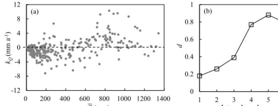
in the 291 study catchments. At the significance level of 0.05, 39.9 % (or 116 of 291) of the study catchments are undergo-ing significant changes in annualQ. These catchments are hereafter referred to as significant catchments. Trends to-wards wetter conditions (positive trends) were found mainly in the upper and lower reaches of the Yangtze River basin and in the basins of the southwest, southeast, Pearl, and In-land rivers. The annualQin the lower reaches of the Yangtze River basin and the northern Xinjiang Uyghur Autonomous Region robustly increased by more than 2 mm a−1, which was greater than the rates of most other catchments. The largest increasing trend of 10.3 mm a−1was observed in the Yangtze River basin. However, the catchments in the mid-dle reaches of the Yangtze River basin and in northern and northeastern China experienced the greatest reductions in runoff, generally with significant trends. Several catchments had negative trends of over 4 mm a−1; the most severe sit-uation was in the Yellow River basin, where the annualQ decreased at a rate of 7.2 mm a−1.
The relationship betweenkQ andQis plotted in Fig. 4,
-12 -8 -4 0 4 8 12
0 200 400 600 800 1000 1200 1400
Q(mm)
kQ
(m
m
a
-1)
0 0.2 0.4 0.6 0.8 1
1 2 3 4 5 6
Interval number
d
(a) (b)
Figure 4. (a)Relationship between observed runoff trendskQand mean annual runoffQfor the study catchments during the period 1956– 2000.(b)Values ofdin each interval according toQ.ddenotes the proportion of catchments with positive trends in each interval. Interval numbers 1 to 6 correspond to six intervals of 0–200, 200–400, 400–600, 600–800, 800–1000, and 1000–1400, respectively.
-9 -6 -3 0 3 6 9 12
0 1 2 3 4 5 6 7 8
kQ
(m
m
a
-1)
φ
0 0.2 0.4 0.6 0.8 1
1 2 3 4 5 6
Interval number
d
(a) (b)
Figure 5. (a)Relationship between observed runoff trendskQand aridity indexϕfor the study catchments during the period 1956–2000. (b)Values ofd in each interval according toϕ. Interval numbers 1 to 6 correspond to six intervals of 0.5–2/3, 2/3–1, 1–1.5, 1.5–2, 2–3, and 3–8, respectively.
Figure 6. (a) Relationship between mean annual runoffQ and aridity indexϕ in the study catchments during the period 1956–2000. (b) Distribution of catchments withϕ >2 and kQ>0. Presenting glaciers are based on the second glacier inventory data set of China (Guo et al., 2014).
catchments became wetter, and the driest catchments became drier.
The DDWW pattern was also examined on the basis of kQ andϕ data. Figure 5 shows thatd decreased from 0.86
to 0.16 asϕ increased, which implies that the DDWW pat-tern also holds if we adopt ϕ to describe the aridity degree in a manner similar to that reported by Greve et al. (2014). This result can be attributed to the monotonic decrease in
Qwithϕ (Fig. 6a). However,dincreased sharply to 0.36 in the last interval, in contrast to the DDWW pattern. To under-stand this divergence, we marked 26 total areas ofϕ >2 and kQ>0 in Fig. 6b. Surprisingly, most of these areas (19 of
[image:6.612.156.436.71.178.2] [image:6.612.157.439.240.353.2] [image:6.612.132.467.418.551.2]y = 0.5379x + 0.5507 R² = 0.7183 -10
-5 0 5 10 15
-10 -5 0 5 10 15
k Q
e
(m
m
a
-1)
kQ(mm a-1)
y = 0.5432x + 0.4744 R² = 0.8813 -10
-5 0 5 10 15
-10 -5 0 5 10 15
k Q
e
(m
m
a
-1)
kQ(mm a-1)
(a) All catchments (b) Significant catchments
[image:7.612.159.440.67.207.2]Error rate: 18.6% Error rate: 6.0%
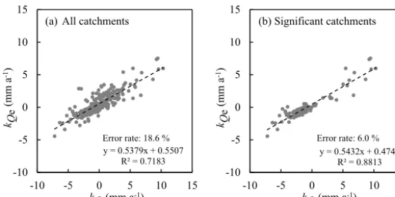
Figure 7.Comparison of estimated runoff trendskQe with observed trendskQfor(a)all catchments and(b)significant catchments.
Sig-nificant catchments are those experiencing sigSig-nificant changes in runoff at the significance level of 0.05. The error rate is defined as the proportion of catchments in which the signs of the observed and estimated trends differ.
Table 2.Number of catchments withkQ>0 and respectivedin each interval based on Q and ϕ in the analysis of the observed trends. Interval numbers based onQandϕare consistent with those in Table 1, as are the interval range and the sample size of each in-terval.dis the proportion of catchments becoming wetter in each interval.
Interval Number of d
number catchments
withkQ>0
Based onQ
1 26 0.18
2 11 0.26
3 12 0.39
4 20 0.77
5 28 0.88
6 15 0.79
Based onϕ
1 18 0.86
2 53 0.74
3 6 0.18
4 9 0.16
5 11 0.16
6 15 0.36
thereby leading to an overestimate of the aridity degree in these catchments caused by grouped into the wrong intervals. This reflects the weakness ofϕin assessing the aridity degree with respect to water resources compared withQ. Moreover, by acquiring 1S and redefining an adjustable aridity index (ϕ0) as (P−1S)/Ep, these catchments with high ϕ could also obey the DDWW pattern.
3.2 Interpreting trends from the climate change perspective
Based on the comparison of the Budyko-estimatedkQe with
the observed kQ, the coefficients of determination (R2)
(Legates and McCabe, 1999) were determined to be 0.70 and 0.86 for all catchments and for significant catchments, respectively (Fig. 7). Therefore, the majority of the runoff trends can be attributed to changes in the atmospheric forcing of water and energy. However, the slope ofkwas smaller than 1, at 0.60 and 0.62 for all catchments and significant catch-ments, respectively, which implies that the Budyko-based framework underestimates the changes in runoff. Neverthe-less, despite underestimating the runoff trends, the frame-work can correctly note the direction of runoff changes in more than 80 % of the study catchments (Fig. 7). This is because the error rates in all and significant catchments, or the proportions of misestimated catchments having different signs of the observed and the estimated trends, are 18.6 and 6.0 %, representing 54 of 291 and 7 of 116, respectively. Furthermore, the DDWW pattern works well based onkQe
(Fig. 8), which validates the DDWW pattern from the per-spective of climate change based on historical meteorologi-cal observations. It also indicates the feasibility of using only P andEpinformation to examine the pattern and serves as a reference for studies based on climate model outputs.
In catchments where the observed and the estimated signs are consistent, the parts of kQe generated from P
(kPQ,=εPkP) andEp(kQ0,=ε0kEp) were compared to find
the factor controlling the runoff changes owing to climate change. As shown in Fig. 9,kP makes an overwhelming
con-tribution in 88.6 % (or 210 of 237) of these catchments be-cause the ratios of absolute k0Q to absolutekQP are smaller than 1. Moreover, when linkingkP withQ(Fig. 10), we
[image:7.612.104.228.350.568.2]-8 -4 0 4 8 12
0 200 400 600 800 1000 1200 1400
0.00 0.20 0.40 0.60 0.80 1.00
1 2 3 4 5 6
kQe
(mm
a
-1 )
Q (mm)
d
Interval number (b)
(a)
Figure 8. (a)Relationship between estimated runoff trendskQeand mean annual runoffQfor the study catchments during the period 1956–
2000.(b)Values ofd in each interval according toQ. Interval numbers 1 to 6 correspond to six intervals of 0–200, 200–400, 400–600, 600–800, 800–1000, and 1000–1400, respectively.
0.0001 0.001 0.01 0.1 1 10
1 10 100 1000 10000
k Q
0/
k Q
P
0 0.2 0.4 0.6 0.8 1
0.0001 0.001 0.01 0.1 1 10
Cu
m
ula
ti
ve frequenc
y
Q (mm) kQ
0
/kQ P
[image:8.612.159.438.69.179.2](a) (b)
Figure 9.Analysis of the controlling factor in the DDWW pattern according to the Budyko hypothesis.(a)Relationship between the ratio of absolutek0Q(=ε0kEp, the part of the estimated runoff trendskQegenerated from potential evapotranspiration changes) to absolutek
P
Q (=εPkP, the part ofkQegenerated from precipitation changes) and the mean annual runoffQ.(b)Cumulative frequency curve of|k
0
Q/kPQ|.
-8 -4 0 4 8
0 200 400 600 800 1000 1200 1400
0.00 0.20 0.40 0.60 0.80 1.00
1 2 3 4 5 6
kP
(mm
a
-1 )
Q (mm) Interval number
d
(b) (a)
Figure 10. (a)Relationship between observed precipitation trendskPand mean annual runoffQfor the study catchments during the
pe-riod 1956–2000.(b)Values ofdin each interval according toQ. Interval numbers 1 to 6 correspond to six intervals of 0–200, 200–400, 400–600, 600–800, 800–1000, and 1000–1400, respectively.
of kP on the runoff trends. Therefore, from the perspective
of climate change, the more uneven precipitation resulted in more uneven runoff, thereby producing the DDWW pattern. 3.3 Predicting future trends using the GCM
projections
Based on the GCM projections, Eq. (8b) predicts the fu-ture runoff trends 1Qe between the periods 1956–2000
[image:8.612.158.439.239.370.2] [image:8.612.158.436.439.550.2]GFDL-ESM2M HadGEM2-ES IPSL-CM5A-LR MIROC-ESM-CHEM NorESM1-M Model-averaged
-1000 -500 0 500 1000
0 200 400 600 800 1000 1200 1400
Q (mm)
∆
Qe
(m
m
)
0.00 0.20 0.40 0.60 0.80
1 2 3 4 5 6
-1000 -500 0 500 1000
0 200 400 600 800 1000 1200 1400
Q (mm)
∆
Qe
(m
m
)
0.00 0.20 0.40 0.60 0.80
1 2 3 4 5 6
-1000 -500 0 500 1000
0 200 400 600 800 1000 1200 1400
Q (mm)
∆
Qe
(m
m
)
0.00 0.20 0.40 0.60 0.80
1 2 3 4 5 6
d
d
Interval number
Interval number
d
Interval number
(a) (b)
(c) (d)
[image:9.612.140.451.83.388.2](f) (e)
Figure 11.Projections of future trends1Qeunder RCP2.6 (top panels), RCP4.5 (middle panels), and RCP8.5 (bottom panels) scenarios for the period 2001–2050.(a, c, e)Relationship between projected1Qeof the five models and their means and mean annual runoffQ.
(b, d, f)Values ofdin each interval according toQbased on1Qeof the five models and their means. Interval numbers 1 to 6 correspond to six intervals of 0–200, 200–400, 400–600, 600–800, 800–1000, and 1000–1400, respectively.
0.01 0.1 1 10 100
1 10 100 1000 10000 0.01
0.1 1 10 100
1 10 100 1000 10000 0.01
0.1 1 10 100
1 10 100 1000 10000
Q (mm) Q (mm) Q (mm)
Cv vC Cv
(a) (b) (c)
Figure 12.Cvvalues of projected future trends1Qeunder(a)RCP2.6,(b)RCP4.5, and(c)RCP8.5 scenarios.
studies (e.g. Greve et al., 2014; Kumar et al., 2016). How-ever, the proposed DDWW pattern is no longer suitable un-der the three scenarios regardless of the model selected be-causeddecreased asQincreased except for interval 6, which showed an increase in contrast to the DDWW pattern. These results do not imply an obvious alleviation of the uneven wa-ter resource distribution. Conversely, they suggest that most areas of China (more than 60 %, as calculated from Table 3) will experience water resource shortages under the projected
climate changes, whereas the conditions of the driest (inter-val 6) and wettest (inter(inter-val 1) areas will be relatively slight. Furthermore, the main meteorological factor controlling the future trends was identified on the basis of the mean results of the five GCMs. Figure 13 shows that the trend inP (1P ) is no longer the controlling factor because only 40 % of the catchments had
ε01Ep
εP1P
values smaller than 1.
[image:9.612.128.468.459.562.2]0.001 0.01 0.1 1 10 100 1000
1 10 100 1000 10000
0.001 0.01 0.1 1 10 100 1000
1 10 100 1000 10000
0.001 0.01 0.1 1 10 100 1000
1 10 100 1000 10000
Q (mm) Q (mm)
(a)
Q (mm)
ε0
∆
Ep
/
εP
∆
P
ε0
∆
Ep
/
εP
∆
P
ε0
∆
Ep
/
εP
∆
P
[image:10.612.130.468.69.165.2](b) (c)
Figure 13.Analysis of the controlling factor in the projected climate change under(a)RCP2.6,(b)RCP4.5, and(c)RCP8.5 scenarios.
70°E 80°E 90°E 100°E 110°E 120°E 130°E 140°E
60°N
50°N
40°N
30°N
20°N
90° E 100°E 110°E 120°E 130°E 140°E 80° E
70° E 60°N
50°N
40°N
30°N
20°N
70°E 80°E 90°E 100°E 110°E 120°E 130°E 140°E
60°N
50°N
40°N
30°N
20°N
Relative
c
hanges
> 0.4 0.2–0.4 0–0.2 -0.2–0
-0.4–0.2 -0.6– -0.4 < -0.6
(a) RCP2.6
(b) RCP4.5
(c) RCP8.5
Cv < 0.5 0.5 < Cv < 1Figure 14.Spatial distribution of the model-averaged relative changes in mean annual runoffQ(=1Qe/Q) for the period 2001–2050 under
(a)RCP2.6,(b)RCP4.5, and(c)RCP8.5 scenarios.
the three scenarios were similar. Red regions indicate catch-ments in which Q will fall by more than 60 % relative to the historical value; most of these regions are located in the Yellow River basin with relatively high certainty (Cv<0.5). The most severe situation occurred in a catchment situated in the Yangtze River basin, where the runoff is predicted to be nearly zero and theCvwas less than 0.2. In contrast, dark blue areas indicate catchments in whichQis projected to in-crease by more than 40 %. These catchments are located pri-marily in the Inland River basin, except for northwest China, where catchments will suffer from a shortage of fresh water. Instead of continuing to become drier, catchments in north-east and north China are projected to generate more runoff in the future, whereas catchments in the lower reaches of the Yangtze River basin will experience considerable reductions in runoff despite historical increases. These are the most ob-vious distinctions between the projected and historical runoff
changes. Thus, the DDWW pattern failed to accurately char-acterize these future patterns.
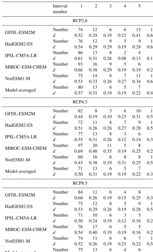
[image:10.612.126.468.202.447.2]Table 3.Numbers of catchments with1Qe>0 and respectivedin each interval based onQof five GCMs and their means in the analysis of the projected trends under three scenarios. Interval numbers based onQandϕare consistent with those in Table 1, as are the interval range and the sample size of each interval.dis the proportion of catchments becoming wetter in each interval.
Interval 1 2 3 4 5 6
number
RCP2.6
GFDL-ESM2M Number 74 12 6 6 13 12
d 0.52 0.29 0.19 0.23 0.41 0.63
HadGEM2-ES Number 76 12 9 5 9 12
d 0.54 0.29 0.29 0.19 0.28 0.63
IPSL-CM5A-LR Number 86 13 8 2 4 3
d 0.61 0.31 0.26 0.08 0.13 0.16
MIROC-ESM-CHEM Number 93 16 9 5 6 4
d 0.66 0.38 0.29 0.19 0.19 0.21
NorESM1-M Number 75 14 8 7 11 13
d 0.53 0.33 0.26 0.27 0.34 0.68
Model-averaged Number 80 13 6 5 7 8
d 0.57 0.31 0.19 0.19 0.22 0.42
RCP4.5
GFDL-ESM2M Number 62 8 3 6 10 11
d 0.44 0.19 0.10 0.23 0.31 0.58
HadGEM2-ES Number 72 11 8 7 9 10
d 0.51 0.26 0.26 0.27 0.28 0.53
IPSL-CM5A-LR Number 77 13 8 3 6 6
d 0.55 0.31 0.26 0.12 0.19 0.32
MIROC-ESM-CHEM Number 97 20 11 5 8 5
d 0.69 0.48 0.35 0.19 0.25 0.26
NorESM1-M Number 60 16 6 8 8 10
d 0.43 0.38 0.19 0.31 0.25 0.53
Model-averaged Number 71 13 6 5 7 7
d 0.50 0.31 0.19 0.19 0.22 0.37
RCP8.5
GFDL-ESM2M Number 84 11 6 4 8 6
d 0.60 0.26 0.19 0.15 0.25 0.32
HadGEM2-ES Number 75 12 8 5 9 10
d 0.53 0.29 0.26 0.19 0.28 0.53
IPSL-CM5A-LR Number 71 10 6 3 5 4
d 0.50 0.24 0.19 0.12 0.16 0.21
MIROC-ESM-CHEM Number 76 17 6 5 5 4
d 0.54 0.40 0.19 0.19 0.16 0.21
NorESM1-M Number 74 11 6 6 7 10
d 0.52 0.26 0.19 0.23 0.22 0.53
Model-averaged Number 75 13 6 4 6 6
d 0.53 0.31 0.19 0.15 0.19 0.32
4 Discussion
In the present work, a new method which is not limited to the artificial selection of the threshold to partition dry and wet regions was proposed to examine the DDWW pattern. Our results confirm that a feasible DDWW pattern exists in the historical runoff trends across China. However, if we adopt the same thresholdϕ=2 as in the study of Greve et al. (2014)
Neverthe-0 500 1000 1500 2000
0 500 1000 1500 2000
Mod
el
led (m
m
)
Observed (mm)
0 500 1000 1500 2000
0 500 1000 1500 2000
Mod
el
le
d
(m
m
)
Observed (mm)
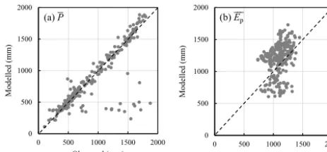
[image:12.612.50.282.67.175.2](a) P (b) Ep
Figure 15. Comparison of the observed meteorological data with the simulations from the GFDL-ESM2M model for the pe-riod 1956–2000.(a)Mean annual precipitationP and(b)mean an-nual potential evapotranspirationEp.
less, from the perspective of the new method, the relationship appears to be consistent with the DDWW pattern including the possibility of 1(P−E) >0 becoming larger asP−E increases. Additionally, the DDWW pattern might also hold in the study of Greve et al. (2014) according to Fig. 4c in that study and the distribution ofϕacross the world. There-fore, a follow-up study will adapt the proposed method to the worldwide scale to examine the DDWW pattern globally.
Based on a Budyko-based framework, our findings suggest that climate change is the main factor of the historical runoff trends in China and thatkP is the most significant factor
as-sociated with climate change. Roderick et al. (2014) reported a similar result in their research of GCM outputs (CMIP3) such that the changes in water availability (1(P−E)) are dominated by the changes inP (1P )globally. Despite high correlation between kQ andkQe, the Budyko-based
frame-work underestimated the observed changes in runoff. This is because the framework quantifies only the effects of cli-mate change. The esticli-mated deviations may stem from the neglect of other influencing factors such as ecological and environmental changes, which result in changes in the catch-ment properties (dnin Eq. 6) which were assumed in this study to be constant.
In this study,Epwas calculated by using the Penman equa-tion, which is considered to be the most effective method (Zhang et al., 2001) and is strongly recommended by Shut-tleworth (2012). This method for estimating Ep was also adopted by other studies such as Yang et al. (2014) and Xu et al. (2015). However, Roderick et al. (2015) suggested using net radiation instead ofEpin the Budyko hypothesis. Kumar et al. (2016) compared runoff change projections obtained by these two different methods and found similar results. There-fore, it is likely that the use ofEpor net radiation had little influence in our results.
Great discrepancy was noted between the GCM-simulated and observedEp, whereas GCM-simulated and observedP showed significant agreement (Fig. 15). This substantial dis-tinction in GCM performance in the P andEpsimulations might evoke doubt about the reliability of the bias-corrected
GCM outputs used in this study. Actually, the bias-correction process was implemented for all GCM outputs, which means that all variables required for calculatingEpwere corrected simultaneously. We speculate that this factor might relate to the disparate effectiveness of the bias-correction process in the different outputs, resulting in a good fit toP and a bad fit toEp.
5 Conclusions
Based on the analysis of restored discharge in 291 catch-ments across China from 1956 to 2000, this study proposed a suitable DDWW pattern of drier regions being more likely to become drier, and wetter regions being more likely to become wetter, which implies that the distribution of water resources in China has become increasingly uneven since the 1950s. This pattern holds in studies adopting both Q andϕ as the indicators of water availability. Furthermore, a framework based on the Budyko hypothesis revealed that the runoff changes can be attributed mainly to climate change and thatkP is the controlling factor. According to the
pro-jections of five GCMs from CMIP5 during the period 2001– 2050, the proposed DDWW pattern is no longer suitable. The model-averaged results suggest that more than 60 % of catch-ments will experience water resource shortages under future climate change. In addition, only 40 % of the study catch-ments will be primarily controlled by1P, which is different from the phenomenon where the runoff change is controlled by precipitation in about 90 % catchments in the historical period. The catchments in northeast and north China, which have become drier, will generate more runoff in the future; those in the lower reaches of the Yangtze River basin, which have become wetter, will experience considerable reductions in runoff. These changes represent the most obvious differ-ences between the projected and historical runoff changes. Nevertheless, the projected conclusions remain tentative ow-ing to the enormous unreliability of the GCM outputs as in-dicated by the extremely low correlations between the simu-lated and observedEpvalues for the period 1956–2000.
Appendix A: Estimate ofEpby the Penman equation
The procedure for using the Penman equation to estimateEp (mm day−1) based on the GCM outputs is described in de-tail in this appendix. The Penman equation can be written as (Yang and Yang, 2011)
Ep=
0.4081 (Rn−G)+2.624γ (1+0.536u2) (1−RH)es
1+γ , (A1)
where es is the saturated vapour pressure (kPa), 1 is the slope of the saturated vapour pressure versus the air temper-ature curve (kPa◦C−1) when the saturated vapour pressure equals es,Rnis the net radiation (MJ m−2day−1),Gis the soil heat flux (MJ m−2day−1),γ is a psychometric constant (kPa◦C−1),u
2is the wind speed at a height of 2 m (m s−1), and RH is the relative humidity (%) (Yang and Yang, 2011).
The form of the saturated vapour pressure versus the air temperature curve is
e(T )=0.6108 exp
17.27T T+237.3
, (A2)
whereT denotes the daily air temperature, andesof the day can be calculated by
es=
e (Tmax)+e (Tmin)
2 , (A3)
whereTmaxandTminare maximum and minimum daily air temperatures, respectively.
The GCM outputs are dailyTmax,Tmin(which can be used to calculatees and1),u2, and RH. AssumingGequals 0, and if we computeRn, we can use Eq. (A1) to estimateEp. The process of utilizing the solar radiation (Rs) to compute Rnis described below.
Firstly, we calculate the incoming net short-wave radia-tion (Rns) by
Rns=(1−α)Rs, (A4)
whereαdenotes the albedo.
Next, the net outgoing long-wave radiation (Rnl) is esti-mated by
Rnl=σ
Tmax4 +Tmin4 2
!
0.34−0.14√ea
1.35Rs Rs0
−0.35
, (A5)
where σ is the Stefan–Boltzmann constant (=4.903×10⁻⁹MJ K−4m−2day−1), ea is the actual vapour pressure (=es×RH), andRs0 is the clear-sky solar
radiation, which can be computed by
Rs0=
0.75+2×10⁻⁵zRa, (A6) wherezis the station elevation above sea level (m), which is available from the GCMs, andRais the extraterrestrial ra-diation (MJ m−2day−1) determined by Eqs. (21) to (25) in Allen et al. (1998).
Finally, by subtractingRnlfromRns, we obtainRn.
Appendix B: Derivation of framework for estimating
kQand1Q
This appendix provides an explicit description of the deriva-tion of the framework for estimating kQ and 1Q from
Eq. (8). Substituting Eq. (8) into Eq. (2) yields
kQ= m P i=1
ti−t
εP1Pi+ε01Epi
m P i=1
ti−t 2
. (B1)
This equation can be transformed into
kQ=εP m P
i=
ti−t1Pi
m P i=1
ti−t
2
+ε0
m P i=1
ti−t1Epi m
P i=1
ti−t
2
. (B2)
Recalling the definition of the trend in this study, Eq. (B2) can be considered as a linear combination ofkP andkEp:
kQ=εPkP+ε0kEp.
Equation (3) can be rewritten as
1Q=
m P i=1
Qpi−mQ
m . (B3)
Recombination of the variables leads to the following expres-sion:
1Q=
m P i=1
Qpi−Q
m . (B4)
Similarly, the substitution of Eq. (8) yields
1Q=
m P i=1
εP1Pi+ε01Epi
m . (B5)
The Supplement related to this article is available online at doi:10.5194/hess-21-2233-2017-supplement.
Competing interests. The authors declare that they have no conflict of interest.
Acknowledgements. This research was partly supported by funding from the National Natural Science Foundation of China (grant nos. 51622903 and 51379098), the National Program for Support of Top-Notch Young Professionals, and the Program from the State Key Laboratory of Hydro-Science and Engineering of China (grant nos. sklhse-2016-A-02 and 2017-KY-01). The authors are grateful to the editor, Jan Seibert, as well as Michael Roderick and the other anonymous referee for providing helpful comments.
Edited by: J. Seibert
Reviewed by: M. Roderick and one anonymous referee
References
Alkama, R., Marchand, L., Ribes, A., and Decharme, B.: Detec-tion of global runoff changes: results from observaDetec-tions and CMIP5 experiments, Hydrol. Earth Syst. Sci., 17, 2967–2979, doi:10.5194/hess-17-2967-2013, 2013.
Allan, R. P., Soden, B. J., John, V. O., Ingram, W., and Good, P.: Current changes in tropical precipitation, Environ. Res. Lett., 5, 025205, doi:10.1088/1748-9326/5/2/025205, 2010.
Allen, R. G., Pereira, L. S., Raes, D., and Smith, M.: Crop evap-otranspiration – Guidelines for computing crop water require-ments, FAO Irrigation and drainage paper 56, FAO, Rome, 1998. Arnell, N. W.: Climate change and global water resources, Global
Environ. Change, 9, S31–S49, 1999.
Budyko, M. I.: Evaporation under Natural Conditions, Israel Pro-gram for Scientific Translations, Jerusalem, 1948.
Chou, C. and Neelin, J. D.: Mechanisms of global warming impacts on regional tropical precipitation, J. Climate, 17, 2688–2701, doi:10.1175/1520-0442(2004)017<2688:MOGWIO>2.0.CO;2, 2004.
Chou, C., Neelin, J. D., Chen, C., and Tu, J.: Evaluating the “Rich-Get-Richer” Mechanism in Tropical Precipitation Change under Global Warming, J. Climate, 22, 1982–2005, doi:10.1175/2008JCLI2471.1, 2009.
Chou, C., Chiang, J. C. H., Lan, C., Chung, C., Liao, Y., and Lee, C.: Increase in the range between wet and dry season precipitation, Nat. Geosci., 6, 263–267, doi:10.1038/ngeo1744, 2013. Choudhury, B. J.: Evaluation of an empirical equation for annual
evaporation using field observations and results from a bio-physical model, J. Hydrol., 216, 99–110, doi:10.1016/S0022-1694(98)00293-5, 1999.
Dai, A., Qian, T., Trenberth, K. E., and Milliman, J. D.: Changes in continental freshwater discharge from 1948 to 2004, J. Climate, 22, 2773–2792, doi:10.1175/2008JCLI2592.1, 2009.
Durack, P. J., Wijffels, S. E., and Matear, R. J.: Ocean Salinities Reveal Strong Global Water Cycle Intensification During 1950 to 2000, Science, 336, 455–458, doi:10.1126/science.1212222, 2012.
Fu, B.: On the calculation of the evaporation from land surface, Sci-enta Atmos. Sin., 5, 23–31, 1981.
Greve, P., Orlowsky, B., Mueller, B., Sheffield, J., Reichstein, M., and Seneviratne, S. I.: Global assessment of trends in wetting and drying over land, Nat. Geosci., 7, 716–721, doi:10.1038/ngeo2247, 2014.
Guo, W., Liu, S., Yao, X., Xu, J., Shangguan, D., Wu, L., Zhao, J., Liu, Q., Jiang, Z., Wei, J., Bao, W., Yu, P., Ding, L., Li, G., Li, P., Ge, C., and Wang, Y.: The second glacier inventory dataset of China (Version 1.0), Cold and Arid Regions Science Data Center, Lanzhou, doi:10.3972/glacier.001.2013.db, 2014.
Hagemann, S., Chen, C., Haerter, J. O., Heinke, J., Gerten, D., and Piani, C.: Impact of a statistical bias correction on the projected hydrological changes obtained from three GCMs and two hydrol-ogy models, J. Hydrometeorol., 12, 556–578, 2011.
Hamlet, A. F., Mote, P. W., Clark, M. P., and Lettenmaier, D. P.: Twentieth-century trends in runoff, evapotranspiration, and soil moisture in the Western United States, J. Climate, 20, 1468– 1486, doi:10.1175/JCLI4051.1, 2007.
Held, I. M. and Soden, B. J.: Robust responses of the hydro-logical cycle to global warming, J. Climate, 19, 5686–5699, doi:10.1175/JCLI3990.1, 2006.
Koster, R. D. and Suarez, M. J.: A simple framework for examining the interannual variability of land surface mois-ture fluxes, J. Climate, 12, 1911–1917, doi:10.1175/1520-0442(1999)012<1911:ASFFET>2.0.CO;2, 1999.
Kumar, S., Zwiers, F., Dirmeyer, P. A., Lawrence, D. M., Shrestha, R., and Werner, A. T.: Terrestrial contribution to the heterogene-ity in hydrological changes under global warming, Water Resour. Res., 52, 3127–3142, doi:10.1002/2016WR018607, 2016. Legates, D. R. and McCabe, G. J.: Evaluating the use
of “goodness-of-fit” measures in hydrologic and hydrocli-matic model validation, Water Resour. Res., 35, 233–241, doi:10.1029/1998WR900018, 1999.
Lim, W. H. and Roderick, M. L.: An atlas of the global water cycle: based on the IPCC AR4 Models, Australian National University Press, Canberra, 2009.
Liu, C., and Allan, R. P.: Observed and simulated precipitation re-sponses in wet and dry regions 1850–2100, Environ. Res. Lett., 8, 034002, doi:10.1088/1748-9326/8/3/034002, 2013.
Milly, P. C. D., Dunne, K. A., and Vecchia, A. V.: Global pattern of trends in streamflow and water availability in a changing climate, Nature, 438, 347–350, doi:10.1038/nature04312, 2005. Oudin, L., Andréassian, V., Lerat, J., and Michel, C.: Has land cover
a significant impact on mean annual streamflow? An interna-tional assessment using 1508 catchments, J. Hydrol., 357, 303– 316, doi:10.1016/j.jhydrol.2008.05.021, 2008.
Pasquini, A. I. and Depetris, P. J.: Discharge trends and flow dynamics of South American rivers draining the southern Atlantic seaboard: an overview, J. Hydrol., 333, 385–399, doi:10.1016/j.jhydrol.2006.09.005, 2007.
Penman, H. L.: Natural evaporation from open water,
bare soil and grass, P. Roy. Soc. A, 193, 120–145,
doi:10.1098/rspa.1948.0037, 1948.
Piao, S., Ciais, P., Huang, Y., Shen, Z., Peng, S., Li, J., Zhou, L., Liu, H., Ma, Y., Ding, Y., Friedlingstein, P., Liu, C., Tan, K., Yu, Y., Zhang, T., and Fang, J.: The impacts of climate change on water resources and agriculture in China, Nature, 467, 43–51, doi:10.1038/nature09364, 2010.
Pike, J. G.: The estimation of annual run-off from meteorological data in a tropical climate, J. Hydrol., 2, 116–123, 1964. Roderick, M. L. and Farquhar, G. D.: A simple framework for
re-lating variations in runoff to variations in climatic conditions and catchment properties, Water Resour. Res., 47, W00G07, doi:10.1029/2010WR009826, 2011.
Roderick, M. L., Sun, F., Lim, W. H., and Farquhar, G. D.: A general framework for understanding the response of the water cycle to global warming over land and ocean, Hydrol. Earth Syst. Sci., 18, 1575–1589, doi:10.5194/hess-18-1575-2014, 2014. Roderick, M. L., Greve, P., and Farquhar, G. D.: On the assessment
of aridity with changes in atmospheric CO2, Water Resour. Res.,
51, 5450–5463, doi:10.1002/2015WR017031, 2015.
Shuttleworth, W. J.: Daily estimates of evaporation, in: Terres-trial Hydrometeorology, John Wiley, Chichester, UK, 334–358, doi:10.1002/9781119951933, 2012.
Stahl, K., Hisdal, H., Hannaford, J., Tallaksen, L. M., van Lanen, H. A. J., Sauquet, E., Demuth, S., Fendekova, M., and Jódar, J.: Streamflow trends in Europe: evidence from a dataset of near-natural catchments, Hydrol. Earth Syst. Sci., 14, 2367–2382, doi:10.5194/hess-14-2367-2010, 2010.
Teng, J., Chiew, F. H. S., Vaze, J., Marvanek, S., and Kirono, D. G. C.: Estimation of climate change impact on mean annual runoff across continental Australia using Budyko and Fu equa-tions and hydrological models, J. Hydrometeorol., 13, 1094– 1106, doi:10.1175/JHM-D-11-097.1, 2012.
Wang, D. and Tang, Y.: A one-parameter Budyko model for wa-ter balance captures emergent behavior in Darwinian hydrologic models, Geophys. Res. Lett., 41, 4569–4577, 2014.
Xiong, L. and Guo, S.: Appraisal of Budyko formula in calculating long-term water balance in humid watersheds of southern China, Hydrol. Process., 26, 1370–1378, doi:10.1002/hyp.8273, 2012.
Xu, K., Yang, D., Yang, H., Li, Z., Qin, Y., and Shen, Y.: Spatio-temporal variation of drought in China during 1961– 2012: A climatic perspective, J. Hydrol., 526, 253–264, doi:10.1016/j.jhydrol.2014.09.047, 2015.
Xu, X., Yang, D., Yang, H., and Lei, H.: Attribution analysis based on the Budyko hypothesis for detecting the dominant cause of runoff decline in Haihe basin, J. Hydrol., 510, 530–540, doi:10.1016/j.jhydrol.2013.12.052, 2014.
Yang, D., Sun, F., Liu, Z., Cong, Z., Ni, G., and Lei, Z.: Analyz-ing spatial and temporal variability of annual water-energy bal-ance in nonhumid regions of China using the Budyko hypothesis, Water Resour. Res., 43, W04426, doi:10.1029/2006WR005224, 2007.
Yang, H. and Yang, D.: Derivation of climate elasticity of runoff to assess the effects of climate change on annual runoff, Water Resour. Res., 47, W07526, doi:10.1029/2010WR009287, 2011. Yang, H., Yang, D., Lei, Z., and Sun, F.: New analytical derivation
of the mean annual water-energy balance equation, Water Re-sour. Res., 44, W03410, doi:10.1029/2007WR006135, 2008. Yang, H., Qi, J., Xu, X., Yang, D., and Lv, H.: The
re-gional variation in climate elasticity and climate contri-bution to runoff across China, J. Hydrol., 517, 607–616, doi:10.1016/j.jhydrol.2014.05.062 ,2014.
Zhang, L., Dawes, W. R., and Walker, G. R.: Response of mean an-nual evapotranspiration to vegetation changes at catchment scale, Water Resour. Res., 37, 701–708, doi:10.1029/2000WR900325, 2001.
Zhang, L., Potter, N., Hickel, K., Zhang, Y., and Shao, Q.: Water balance modeling over variable time scales based on the Budyko framework – model development and testing, J. Hydrol., 360, 117–131, doi:10.1016/j.jhydrol.2008.07.021, 2008.