A case study of field scale maize irrigation patterns in western Nebraska: implications for water managers and recommendations for hyper resolution land surface modeling

www.hydrol-earth-syst-sci.net/21/1051/2017/ doi:10.5194/hess-21-1051-2017

© Author(s) 2017. CC Attribution 3.0 License.

A case study of field-scale maize irrigation patterns in western

Nebraska: implications for water managers and recommendations

for hyper-resolution land surface modeling

Justin Gibson1, Trenton E. Franz1, Tiejun Wang1,2, John Gates3, Patricio Grassini4, Haishun Yang4, and Dean Eisenhauer5

1_{School of Natural Resources, University of Nebraska-Lincoln, Lincoln, NE, USA}

2_{Institute of Surface-Earth System Science, Tianjin University, Tianjin 300072, P. R. China} 3_{The Climate Corporation, San Francisco, CA, USA}

4_{Department of Agronomy and Horticulture, University of Nebraska-Lincoln, Lincoln, NE, USA} 5_{Biological Systems Engineering Department, University of Nebraska-Lincoln, Lincoln, NE, USA}

Correspondence to:Trenton E. Franz ([email protected]) and Justin Gibson ([email protected]) Received: 26 August 2016 – Discussion started: 30 August 2016

Revised: 9 December 2016 – Accepted: 31 January 2017 – Published: 20 February 2017

Abstract.In many agricultural regions, the human use of wa-ter for irrigation is often ignored or poorly represented in land surface models (LSMs) and operational forecasts. Because irrigation increases soil moisture, feedback on the surface energy balance, rainfall recycling, and atmospheric dynam-ics is not represented and may lead to reduced model skill. In this work, we describe four plausible and relatively simple irrigation routines that can be coupled to the next generation of hyper-resolution LSMs operating at scales of 1 km or less. The irrigation output from the four routines (crop model, pre-cipitation delayed, evapotranspiration replacement, and va-dose zone model) is compared against a historical field-scale irrigation database (2008–2014) from a 35 km2 study area under maize production and center pivot irrigation in western Nebraska (USA). We find that the most yield-conservative irrigation routine (crop model) produces seasonal totals of irrigation that compare well against the observed irrigation amounts across a range of wet and dry years but with a low bias of 80 mm yr−1. The most aggressive irrigation sav-ing routine (vadose zone model) indicates a potential irriga-tion savings of 120 mm yr−1 and yield losses of less than 3 % against the crop model benchmark and historical aver-ages. The results of the various irrigation routines and asso-ciated yield penalties will be valuable for future considera-tion by local water managers to be informed about the po-tential value of irrigation saving technologies and irrigation

practices. Moreover, the routines offer the hyper-resolution LSM community a range of irrigation routines to better con-strain irrigation decision-making at critical temporal (daily) and spatial scales (<1 km).

1 Introduction

irri-gation databases ( Grassini et al., 2011, 2014, 2015), mostly focusing on benchmarking on-farm irrigation in relation to crop production.

With the continual refinement in the spatial resolution of LSMs down to<1 km (Wood et al., 2011) and the coupling to crop models (Kucharik, 2003), reliable irrigation data need to be incorporated in the calibration and validation of LSMs. Although the presence of irrigation does not necessarily im-pact soil moisture contribution to the atmosphere, the soil moisture–flux relationship is critical to surface energy bal-ance and atmospheric dynamics. One area of particular im-portance is the impact of soil moisture on atmospheric pro-cesses, such as rainfall recycling (Findell and Eltahir, 1997), the strength of atmospheric coupling (Koster et al., 2004), and planetary boundary layer dynamics (Santanello et al., 2011), all of which impact the skill in operational forecast models. More complicated is that both irrigation timing and volumes are based on human decision-making processes and biophysical requirements (Gibson, 2016). For example, the USDA found that 24 % of producers relied on crop calendars, 16 % on crop consultants, and 23 % on in situ probe technol-ogy (USDA, 2014). Because irrigation decisions are depen-dent on both processes, reliable historical irrigation data are critical to understand why and how decisions were made in order to accurately represent the physics in hyper-resolution LSMs and operational forecast models. In the absence of irri-gation data, LSMs have typically relied on mass balance ap-proaches (Döll and Siebert, 2002; Wada et al., 2012) where irrigation amounts close the water balance. While a reason-able first approach, this methodology may introduce addi-tional uncertainty into LSMs due to the complexity of rep-resenting the human decision-making process on water use. The uncertain irrigation schemes affect the time history of soil moisture and thus our ability to properly assess the impacts of human water use on coupled land–atmospheric model physics.

The focus of this study was to investigate historical irri-gation use at the critical field scale (∼0.8 by 0.8 km) in a study area of 3500 ha in western Nebraska, which sits on the edge of the US Corn Belt. This critical scale is defined as a point where human water decisions are made due to the history of land partitioning and the inherent geometry dic-tated by the landscape. While it is a relatively small area, the study site is an ideal location for assessing the sustain-ability of groundwater pumping for the irrigation of crops. The study area is a microcosm of many areas across the globe, where humans rely on groundwater withdrawals for their livelihoods (Mekonnen and Hoekstra, 2011). The study area is at a critical location on a boundary where irrigation supply volumes can no longer economically compensate for the deficit between potential evapotranspiration (ETp) and

precipitation (P). Of particular concern regarding impacts on both human and natural ecosystems are the resultant de-clines in the local water table due to irrigation (Young et al., 2014). For example, the southern portion of the High

Plains aquifer (HPA) has had significant groundwater deple-tion over the last 80 years, with losses of up to 50 % in sat-urated thickness (Scanlon et al., 2012). In the northern HPA (Butler et al., 2016), where this study area is located, intense irrigation pumping has led to localized water table declines (specifically in Box Butte County and widespread throughout the neighboring Upper Republican Natural Resources Dis-trict) but has yet to be widespread across the region (Young et al., 2013). Given low recharge (Szilágyi and Jozsa, 2013; Gibson, 2015; Wang et al., 2016) relative to irrigation pump-ing, rising global food and water demands (FAO, 2009), and the concomitant effects of climate change (Kumar, 2012), the sustainability of this study area and the overall HPA sys-tem in support of long-term irrigation agriculture is uncertain (Butler et al., 2016). The study presented here is an important first step in assessing water-saving technologies to continue to make irrigation agriculture sustainable; there is a critical need for this in meeting rising global food demands.

Here, we benchmark relatively long-term (2008–2014), field-specific flow meter irrigation amounts within the study area against a range of irrigation strategies. The data include information on 55 fields (∼65 ha) producing maize under center pivot irrigation. Datasets at this critical LSM scale are rare due to privacy concerns and, as a result, are often aggre-gated to county and seasonal totals (USDA, 2014; USDA-NASS, 2014). This makes an assessment of irrigation depths over a given area difficult to ascertain. This study therefore fills a critical data need in the development and testing of the next generation of hyper-resolution LSMs and operational weather forecast models (Kumar et al., 2015). The next gen-eration of LSMs will be essential to better assess the impacts of irrigation on the surface energy balance as well as to eval-uate the long-term sustainability of groundwater resources in agricultural areas. We note that irrigation is a key component of global food security, accounting for∼40 % of global food production and ∼20 % of all arable land (Molden, 2007; Schultz et al., 2005). There is no doubt that irrigation will continue to expand in the future.

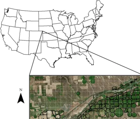
Figure 1.The study area located in western Nebraska with a 1 km grid (white lines) overlaid on the study site. The black lines show the individual field locations where irrigation volumes/depths are obtained from the SPNRD.

well as a strategy for investigating technology adoption sce-narios.

2 Methods

2.1 Description of study area and historical data The study area is located in western Nebraska where the South Platte River enters the state (Fig. 1). The site encom-passes 55 fields with an average area of 65 ha under irrigated maize production (3500 ha total area). Overhead sprinkler irrigation from center pivots using water from the underly-ing HPA is the most common form of irrigation in this area as well as throughout Nebraska and the USA; it is a cost-effective and more efficient option than flood irrigation. The study area is semiarid, and annual crop referenced (maize) evapotranspiration (ETc) is significantly higher than

precip-itation (P) (HPRCC, 2016). The 7-year (2008–2014) aver-age annual P is 440 mm yr−1 and average annual ETc is

820 (mm yr−1), as measured by the High Plains Regional Climate Center weather station (HPRCC, 2016) located within 10 km of the study area near Brule, NE.

Data obtained from SSURGO (Soil Survey Staff, 2016) in-dicate that soil texture in the area falls within two USDA tex-tural classes: sandy loam and loam (Fig. 2). Historical land management data for the area are available from the South Platte Natural Resources District (SPNRD, 2016). The SP-NRD dataset includes field-specific information from 2008– 2014 on crop type, irrigation pumping volumes, and irri-gated area. Detailed descriptions and quality control of NRD databases can be found in Grassini et al. (2014) and Farmaha

Figure 2.The area-weighted soil texture of all fields plotted on the USDA soil texture triangle, falling primarily in the sandy loam and loam textures. Data downloaded from the NRCS Web Soil Survey.

et al. (2016). The above datasets provide the needed meteo-rological forcing, model parameters, and calibration datasets for running and evaluating the suite of irrigation modeling routines described below.

2.2 Irrigation modeling routines

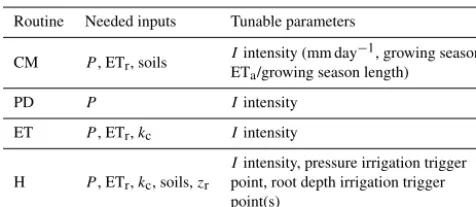
In the following sections, we will describe the four identified irrigation triggering routines: crop model (CM), precipita-tion delayed (PD), evapotranspiraprecipita-tion replacement (ET), and Hydrus-1D (H). The four irrigation triggering routines rep-resent the upper limit of irrigation requirements, in which no plant water stress occurs (CM), and the lower irrigation limit needed to ensure minimal yield loss against a crop model benchmark (H). Moreover, the four routines can be easily coupled or implemented into LSMs where PD is the simplest routine and H the most complex. We also note that the dif-ference between historical irrigation practices and the lower bound of simulated irrigation provides a potential irrigation savings value in the study area. This irrigation savings value will be important for evaluating the economics of new irri-gation technologies as well as providing critical information to policy makers and local stakeholders on the sustainable management of the HPA (Butler et al., 2016). Table 1 pro-vides a summary of key needed inputs and a list of tunable parameters for each routine.

2.2.1 Crop model irrigation (CM)

wa-Table 1.Summary of needed inputs and tunable parameters for each irrigation routine.

Routine Needed inputs Tunable parameters CM P, ETr, soils Iintensity (mm day

−1_{, growing season}

ETa/growing season length)

PD P Iintensity

ET P, ETr,kc Iintensity

H P, ETr,kc, soils,zr

Iintensity, pressure irrigation trigger point, root depth irrigation trigger point(s)

ter stress. The model performance has been extensively val-idated against measured yield in crops that received near-optimal management across the Corn Belt (Grassini et al., 2009, 2011). However, it has not been rigorously tested for seasonal irrigation totals, which is one key outcome of this study. Details on the model can be found in Yang et al. (2013), and a brief description of the model is given here. Inputs to this model include meteorological data, soil texture, crop biophysical parameters, sowing date, and plant density. The datasets are described above in Sect. 2.1. The soil water dynamics over the root zone are simulated through a bucket model approach with 10 cm thick layers. Drainage between soil layers occurs when soil moisture exceeds field capacity. Irrigation application is triggered when actual ET (ETa) is

less than crop referenced potential evapotranspiration (ETc),

ensuring that no water stress occurs throughout the entire growing season. Irrigation depth is determined by the deficit of soil moisture defined by the current moisture level sub-tracted from 95 % of field capacity within the managed root zone. Maximum water application per irrigation event was set to 19.5 mm. When the depth-weighted unsaturated hy-draulic conductivity (Kr) of the root zone is greater than or

equal to ETc, ETais equal to ETc. Otherwise, ETais equal to

the depth-weightedKrof the root zone.

2.2.2 Precipitation delayed irrigation (PD)

Water application in an idealized land management operation would consider all components of the water balance within the decision-making process. However, in practice, precipi-tation is often the only component considered due to (1) the difficulty of accurately measuring the other water balance components and (2) the minimal relative economic return considering the perceived potential of crop yield loss ver-sus savings due to reduced pumping/irrigation. With this in mind, producers often develop “rules of thumb” to irrigate up to a target total amount of water equal to irrigation plus in-season rainfall (in the study area, 1 May to 30 Septem-ber). Using these basic rules of thumb and local crop cal-endar requirements, we suggest the following routine based on precipitation data alone. However, we note that this is not a recommendation for producer adoption, but instead

represents a simplified method of irrigation management for modeling purposes. In addition, the applicability of this method to other regions should be possible with complemen-tary datasets (i.e.,P and ETc). Recommendations obtained

from the SPNRD indicate that maize requires approximately 650 mm of total water (precipitation plus irrigation,P+I) per growing season (http://www.spnrd.org/index.html). Field observations indicate that irrigation often starts around mid-June and concludes around mid-September, leading to a 100-day irrigation season. Average irrigation application in the absence of precipitation would be 6.5 mm day−1or 19.5 mm per 3-day period. This irrigation depth is consistent with pro-ducer interviews and local expert knowledge. Three-day peri-ods are critical to consider, as this is often the time required to perform a single 360◦rotation of a center pivot (i.e., dictated by soil infiltration rates and well pumping capacity). In this routine, if rainfall is greater than 6.5 mm day−1_{, then}

irriga-tion for 1 day is met, and thus a 1-day delay is set. Likewise, for a rainfall event of 13 mm day−1, then 2 days of irrigation are met and irrigation is delayed by 2 days, and so on for larger rain events. For simplicity, rain events and irrigation delays are rounded to the nearest day and up to a maximum 7-day delay. For rainfall events greater than 45.5 mm day−1, we assume a maximum delay of 7 days due to deep drainage and runoff losses incurred during the event.

2.2.3 ET replacement irrigation (ET)

The primary purpose of irrigation is to ensure that ETais able

to adequately keep up with ETc over the growing season,

as ETa is linearly correlated with yield (Passioura, 1977).

Proper management allows a deficit between applied water and ETain order to allow for adequate infiltration after

rain-fall. The deficit was assumed to be 6.5 mm for this routine based on the average daily crop water requirement discussed above. In this algorithm, when the deficit was greater than 6.5 mm during the irrigation season (15 June to 30 Septem-ber), an irrigation event of 19.5 mm was triggered for the next day. Again, an irrigation event of 19.5 mm was used as it rep-resents a 3-day period over which the center pivot operates.

Estimating ETcis necessary in order to track the deficit

be-tween applied water and ETa. While estimating ETcis

com-plex given the variability of micrometeorological variables from one field to another, in practical applications, crop co-efficients are often used to surmise the differences in crop biophysical relationships and the effect of soil (Shuttleworth, 1993). These coefficients are often published by local ser-vices like the state climate office or the HPRCC in Nebraska. Here, ETc(mm day−1) was estimated by following the

sin-gle crop coefficient method outlined in Allen et al. (1998):

ETc=ETrKc, (1)

where ETr(mm day−1) is reference crop ETpcalculated from

micrometeorological variables and Kc is a dimensionless

well as the average effect of soil on evaporation rates. Daily ETr data were determined from the HPRCC weather

sta-tion data.Kcvalues were calculated as a function of

grow-ing degree day accumulation (GDD) from the HPRCC data (HPRCC, 2016). A single-day calculation of growing de-grees (GDDdaily) is defined as

GDDdaily=

Tmax+Tmin

2 −Tbase, (2)

where Tmax is the daily maximum temperature (◦C) (with

a maximum of 30◦C),Tminis the daily minimum

tempera-ture (◦C), andTbaseis 10◦C. The GDD method is preferred as

it more accurately represents a proxy for crop development, as opposed to a fixed number of days after sowing.

2.2.4 Hydrus-1D irrigation (H)

A physically based vadose zone model, Hydrus-1D (H1D) (Šim˚unek et al., 2013), was used to simulate irrigation re-quirements based on predefined soil pressure head trigger points in the root zone. In order to carry out the neces-sary seasonal dynamics for annual crops (i.e., dynamic root growth, root distribution), we coupled the HM and H1D models using Matlab. We note that soil pressure triggered irrigation events based on more than one soil pressure value, flexible irrigation time frames, and dynamic root growth with a specified distribution are unavailable in the standard H1D code. Here we use Matlab to link together a series of 1-day simulations (totaling 7 years), where model outputs (pres-sure head at depth, flux rates, actual evapotranspiration, etc.) at the end of the day were used to make a decision about irrigation for the following day.

H1D simulates soil water dynamics and water flow with a numerical approximation of the 1D Richards’ equation:

∂θ ∂t =

_∂

∂z K(θ )

_∂h

∂z+1

−S, (3)

whereθ is volumetric water content (cm3cm−3),t is time (day),zis the spatial location (cm),K(h)is unsaturated hy-draulic conductivity (cm day−1),his pressure head (cm), and Sis a sink term describing evapotranspiration (1 day−1). The soil profile simulated is 6 m deep with a 1 cm node discretiza-tion. Free drainage is set for the lower boundary condition, as local depth to groundwater is on average 15 m (Korus et al., 2013)

The H1D model requires that ETcbe partitioned into

po-tential evaporation and popo-tential transpiration. This is accom-plished using Beer’s law:

Tp=ETc

1−e−k·LAI, (4)

Ep=ETc−Tp, (5)

whereTpis potential transpiration (cm day−1),Epis

poten-tial evaporation (cm day−1),kis the light extinction coeffi-cient (set to 0.55; Yang et al., 2013), and LAI (m2m−2) is

the leaf area index. For each year’s growing season, we sim-ulated a daily LAI time series using HM. This same seasonal dynamic was used for all simulations. In addition, HM was used to estimate the date of silking for each simulated year. Water stress is minimized during silking periods, as this is the most critical grain filling period for yield. Most produc-ers will heavily water in this period to ensure yield. In order to accurately represent irrigation behavior, we forced irriga-tion events every 3 days, 1 week before and after the silk-ing date. In cases where a simulated day occurred dursilk-ing the growing season, root depth (Zr, cm) and root

distribu-tion (ZrRD, dimensionless) parameters were calculated on a

daily basis from a predetermined GDD accumulation after the planting date for each growing season. This process was carried out following the equations outlined in the HM user manual (Yang et al., 2013):

Zr=

GDD GDDsilking

Zrmax, (6)

ZrRD=exp(−VDCZL/Zr) , (7)

where GDDsilkingis growing degree days at silking,Zrmax is

a biophysical parameter representing the maximum depth the root zone can reach (in cm) set to 150 cm (Yang et al., 2013), VDC is a vertical distribution coefficient set to 3, andZLis the current depth in the root zone (cm).

Irrigation events and depths for the following day were calculated by investigating the average soil pressure heads at 30, 60, and 90 cm during the historical irrigation period from 15 June through 30 September. Prior to the silking date, the average soil pressure head at 30 and 60 cm is com-puted and compared against a preset irrigation trigger value set to−500 cm based on the dominant soil types in the area (Fig. 2). Following the silking date, the average soil pressure is computed at 30, 60, and 90 cm with the same trigger point of−500 cm of pressure. This algorithm is based on the best practice irrigation recommendations summarized in Irmak et al. (2014). In practice, producers vary the irrigation pressure trigger point based upon farmer risk aversion and soil type. Given that yield is the primary economic driver over energy costs for pumping water, this trigger point is often set at conservative values. When the pressure head at the consid-ered depths exceeds the trigger point, an irrigation event of 19.5 mm is set for the following day. The irrigation event is added to any precipitation that may arrive randomly on that day as well.

Figure 3.Cumulative in-season precipitation depths measured at seven rain gauges and crop referenced evapotranspiration (ETc) calculated

from a weather station<10 km away. Precipitation variability tends to increase with increasing seasonal totals.

zone depth, root distribution, and irrigation amounts were changed for the following day. Using this routine, the model was run continuously at 1-day intervals for the entire study period (1 January 2008 to 31 December 2014).

2.3 Rainfall variability across the study site

Daily precipitation data for the years 2008–2014 were avail-able from seven gauges within a 35 km radius of the study site. In order to help assess the effect of precipitation vari-ability on irrigation application, all seven time series along with the average precipitation time series were used within the four irrigation routines described above. In addition, all irrigation routines that considered soil type were repeated for the two dominant soil types in the study area, i.e., sandy loam and loam.

3 Results

3.1 Precipitation variability and ETc

As expected, significant gauge-to-gauge variability was ob-served within the seven rain gauge time series within each growing season with a mean of 320 mm and a coefficient of variation (CV) of 35 % (Fig. 3). In general, as pre-cipitation totals increased, the range of seasonal precipita-tion totals observed by the seven gauges increased as well (slope=0.246 mm yr−1, R2=0.38). There was no consis-tent year-to-year spatial precipitation gradient, and no gauge consistently reported high or low totals. We hypothesize that this natural variability in rainfall is a large contributor to the irrigation variability we see at the field level. This hypothe-sis was beyond the scope of the current paper, but we

sug-Figure 4.Box and whisker plots of historical irrigation depths for all sites. The upper and lower boundaries of the boxes indicate the 75th and 25th percentile, respectively. The horizontal line within the boxes is the median value. Whiskers are the maximum and min-imum values. Asterisks indicate that irrigation distribution deviates from a normal distribution (D’Agostino–Pearson test,p <0.01).

gest future research in this area (cf. Gibson, 2016). In terms of growing season ETc, the HPRCC reported an average of

815 mm and was within 10 % of the county-level values esti-mated by Sharma and Irmak (2012).

3.2 Historical field-scale irrigation

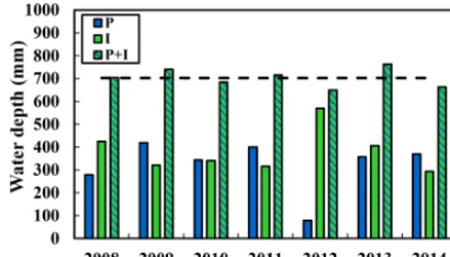
Figure 5.Observed growing season totals for precipitation (P), ir-rigation (I), andP+I. The dashed line represents the historical average forP+I.

found that soil texture was not a significant factor affecting irrigation application at the field scale in this region. This finding was consistent with results from central Nebraska (Gibson, 2016). After grouping the fields by soil type (loam and sandy loam), we found that the irrigation means for all years were not statistically different from each other (Stu-dent’st test,p=0.73). This indicates that soil type did not factor into the irrigation decision-making process.

3.3 Comparison of historical seasonal irrigation amounts with four irrigation routines

The results of the comparison between the historical irriga-tion (2008–2014) and the four irrigairriga-tion routines are summa-rized in Fig. 6. Both the CM and PD routines reproduce the trend of the historical irrigation amounts but with a low off-set (similar slopes). CM irrigation water requirements were on average 80 mm lower (20 % of total) relative to histori-cal irrigation. For PD, the average seasonal difference was 40 mm lower (10 % of total). For ET and H, simulated irriga-tion amounts were 80 mm (20 % of total) and 120 mm (30 % of total) lower than the historical average, respectively. We also note that the slopes of the observed irrigations and the CM and PD for the given years were generally similar. How-ever, it is obvious from Fig. 6 that the slopes of ET and H were different from the observations, which results in larger deviations in drier years and thus a potential for greater irri-gation savings. The implications for water management will be discussed in the next section.

3.4 Irrigation sensitivity to rainfall

All irrigation routines responded to differences in the eight rainfall time series, and this response is represented as ver-tical error bars in Fig. 6. The difference between the highest and lowest irrigation amount for each growing season was on average 75 mm, or 20 % of average irrigation totals. The largest difference in irrigation totals occurred in 2008 for all irrigation routines with an average of 130 mm between all four routines, and the smallest difference occurred in 2012 at

Table 2.The van Genuchten parameters used in the Hydrus-1D sim-ulations.

Texture θr θs α n Ks

(–) (–) (1/cm) (–) (cm day−1) Sandy loam 0.048 0.385 0.0289 1.389 31.91 Loam 0.060 0.400 0.0127 1.458 10.85

an average of 27 mm due to uniformly low precipitation. The analysis illustrates that the variation in irrigation amounts de-pends on which rainfall gauge is used to make a decision. Given that producers often have fields distributed across a region, the uncertainty in local rainfall directly propagates variations in irrigation amounts (Gibson, 2016). Future re-search efforts should investigate the effect of spatial rainfall variability on producer decision-making, but this was beyond the scope of the current study.

3.5 Soil texture impact on irrigation routines

We found that the two dominant soil textures in the study area did not have a significant impact on irrigation amounts under CM and H. ET and PD do not have a soil component considered in their routine and are therefore not impacted by soil texture. In the case of CM, average irrigation was within 1 % for all years. For H, the irrigation average of the sandy loam soil was 10 % lower than the average of the loam soil. The soil hydraulic parameters used for both soil textures were determined using ROSETTA (Schaap et al., 2001) and are presented in Table 2.

3.6 Simulated yield under irrigation routines

Following the simulated irrigation for the routines of PD, ET, and H, the (P+I) time series were reinserted back into the crop model for all years to estimate yield impacts (Fig. 7). The crop model yielded an average of 14.6 Mg ha−1_{over the}

study period. The yield gap (i.e., the difference between yield potential and actual yield) of US irrigated maize represents approximately 15 % of the potential (Grassini et al., 2013; Global Yield Gap and Water Productivity Atlas, 2016), sug-gesting an average actual yield of 12.4 Mg ha−1for the study area, which is within 5 % of the historically reported yield. For the three routines and for all years, simulated yields were on average within 3 % of the simulated yield based on the CM. The results indicate that the various irrigation schedul-ing strategies did not have a large impact on yield, but they reduced irrigation amounts substantially; hence, they may be a sound economic option for producers.

Figure 6.Historical irrigation vs. the four simulated irrigation routines for sandy loam (left panel) and loam (right panel). The vertical error bars are the standard error of the mean from the precipitation sensitivity analysis, and the horizontal error bars are the standard error of the mean from observed irrigation.

Figure 7.Potential yield simulated by Hybrid-Maize using the four irrigation routines: crop model (CM), precipitation delayed (PD), evapotranspiration replacement (ET), and Hydrus-1D (H).

tends to begin later in the growing season for the two routines that consider soil (CM and H). This is likely due to the rou-tines allowing soil moisture to be depleted before irrigation is triggered, thus creating the reduced pumping and irriga-tion savings. The amount of soil moisture storage is typically near field capacity, but in exceptionally dry years (2012) this storage is reduced and thus will lead to less of a delay at the start of the growing season.

4 Discussion

4.1 Temporal variability of applied irrigation

Historically, the study area has had a consistent amount of total seasonal water (P+I) from year to year. The percent of irrigation to applied water (I /(P+I )) was on average 55 %; notably in 2012, this was as high as 88 %. The relative weight of irrigation to precipitation highlights the importance of constraining irrigation amounts for proper water balance closure within the study area, as well as in other areas with intense irrigation application. Given the high seasonal rates of irrigation to precipitation, no doubt the soil moisture will

be adversely affected when compared to a rainfed area. More importantly, the impacts on the local surface energy balance (Santanello et al., 2011), rainfall recycling, and skill in ob-servational forecasts may be diminished without properly accounting for irrigation. For example, regional mesoscale modeling illustrated that up to 40 % of East African annual rainfall can be attributed to irrigation across India (de Vrese et al., 2016). With the suggested findings here on reduced ir-rigation needs (up to 115 mm or 30 %), the potential changes to precipitation patterns across the HPA due to the adoption of irrigation scheduling technology should be further inves-tigated.

The study area is currently under groundwater appropri-ation, with a historical increase in depth to groundwater of 1.2 m from 1971 to 2013 (SPNRD, 2013; Young et al., 2013). Precipitation pattern changes in the area induced by global warming are believed to lead to less frequent but more in-tense storms with an increase in total precipitation (Dai, 2011). However, the timing of precipitation is of equal con-cern as totals, as more infrequent rain events may still lead to increased pumping with the same seasonal totals. The sce-nario of changing precipitation amounts and timing is not unique to the study area, but it is a more general pattern of the region; this highlights the need for explicit treatment of irrigation depths and timing to fully understand the complex feedback that exists beneath the land surface and atmosphere. The irrigation routines suggested in this work can be used as a first assessment of the likely irrigation amounts due to dif-ferent observed scheduling practices (USDA, 2014). 4.2 Spatial variability of applied irrigation

Figure 8. Example of simulated growing season cumulativeP andP+I with dailyP values plotted on the secondaryy axis for the four irrigation routines in a wet (2010) and dry year (2012). Irrigation starts later for routines that track soil moisture, thus leading to reduced pumping.

year (2012) had the largest standard deviation (168 mm) for applied irrigation. The results are likely due to two reasons: (1) producers give up irrigation at some point during the growing season as their crop parishes in the extreme heat and drought conditions and (2) differences in well-to-well pump-ing capacity become more apparent with increased pumppump-ing demand. Although no direct work has been done to confirm differences in pumping capacity or inefficiencies in the study area, the general effect has been explored through modeling in other areas (Foster et al., 2014). With respect to LSMs, these two factors represent significant deviations from water balance closure approaches, making it challenging to include realistic irrigation values in dry years. Therefore, additional studies and datasets similar to those presented here are crit-ical for the calibration and validation of the next generation of hyper-resolution LSMs.

With regard to soil texture differences in the study area, observed irrigation data indicated no difference between fields in these two texture classes. Similar behavior was seen from the irrigation routine simulations, which showed a 10 % difference for H and a 1 % difference for CM. We note that given the similar soil texture classes (and thus the soil hy-draulic parameters), this result is not unexpected. In practice, producers are beginning to adopt precision irrigation tech-niques (Hedley and Yule, 2009; Hedley et al., 2013). Small-scale features within a field (e.g., sandy or gravelly areas, underperforming parts of the field, waterways, pivot roads, etc.) can be better managed with the new technology. There-fore, managing fields by following one dominant soil type (i.e., irrigation pressure trigger point) may be highly ineffi-cient (Kranz et al., 2014). More refined and consistent soil texture data across arbitrary political boundaries (Chaney et al., 2016) are needed to better account for differences in ir-rigation water application on the subfield scale, especially in areas with increasing adoption of precision agriculture tech-nology.

4.3 Potential for reduced pumping

The four irrigation routines represent different levels of al-lowable water stress that develop in the maize. The CM rou-tine is the lowest risk approach with respect to yield and represents the modeled upper limit of required irrigation to maintain a stress-free management scenario. It is hypothe-sized that any irrigation application above this represents ir-rigation application due to risk aversion and will not appre-ciably increase yield. Comparisons between 2008 and 2014 indicate that the slopes of the applied irrigation from ob-served irrigation are indistinguishable, but with a bias of ∼80 mm yr−1 _{more observed irrigation. This indicates that}

producers are averaging an additional three to four irrigation cycles beyond what the CM indicates. The differences in ir-rigation totals from the other three irir-rigation routines are the result of increasing allowable water deficits in the routines. A reduction of 115 mm or 30 % in irrigation was observed for H when compared to the historical average. We note that this hypothetical scenario requires perfect management with full trust of the technology and may not be achievable in practical applications. However, we anticipate that a 50–75 mm reduc-tion over a short technology adopreduc-tion period (2–4 years) is feasible, particularly in areas with strong university exten-sion programs and/or producer-to-producer knowledge ex-change (Irmak et al., 2012). In addition, these hypothetically reduced pumping numbers may be useful to local, state, and federal policy makers in future water management decisions and investment in cost-sharing technology programs. 4.4 Assessment of center pivot irrigation routines in

hyper-resolution land surface models

that the magnitude of the offset is likely related to local pro-ducer behavior and influenced by social norms and risk aver-sion. Gibson (2016) provides a fuller assessment of irrigation behavior throughout central Nebraska. We note that it is un-clear how these routines would behave in areas with center pivots outside the USA (i.e., Brazil, South Africa, and Aus-tralia), where energy costs for pumping may be more restric-tive drivers of human decisions on irrigation. An assessment of these routines in those areas would require further valida-tion.

We believe that the routines, combined with a reasonable offset correction, could be easily incorporated into future hyper-resolution LSMs with the above routine descriptions and readily available LSM model output or datasets (see Ta-ble 1). Clearly, accurate and local precipitation is critical in driving these irrigation routines and capturing producer be-havior. This topic deserves more research, particularly the opportunity to combine low-cost in situ gauges with radar and remote-sensing products. Additionally, we note that the four routines could be run offline in order to provide reason-able guesses of applied irrigation for a given irrigation sea-son. This may be beneficial in representing processes not ex-plicitly considered in LSMs (Kumar et al., 2015) or making future assessments and recommendations about water avail-ability for managers. Finally, the four routines provide rea-sonable irrigation bounds and, more importantly, predictions about decreases in irrigation as technology is introduced and adopted in novel areas.

5 Conclusions

In this work, we describe four plausible and relatively simple irrigation routines that could be coupled to the next genera-tion of hyper-resolugenera-tion LSMs operating at scales of 1 km or less. The crop model irrigation outputs reproduce the year-to-year variability of the observed irrigation amounts with a low bias of 80 mm yr−1. Predictions from the vadose zone model indicate potential irrigation savings of up to 120 mm yr−1for maize. In addition, daily precipitation variability across the study area was found to introduce significant variability in daily irrigation decision-making depending on which value was considered. Future work could focus on providing ac-curate real-time 1 km daily precipitation products through a combination of in situ low-cost gauges, radar, and satel-lite remote-sensing. Accurate and real-time precipitation re-mains a critical weakness in rural and vast landscapes. Given the clustering of irrigation fields in western Nebraska, the number of in situ gauges needed could be significantly re-duced to provide high-density networks in key areas. The findings from this work may be useful to local water man-agers and stakeholders in evaluating potential water-saving technologies. In addition, the simple routines could be cou-pled to future hyper-resolution land surface models that seek to understand the degree of land–surface atmospheric

cou-pling and the consequences for operational forecasts. This understanding is essential as society continually recognizes the importance of human activities for the global water cycle and invests more resources in understanding the water–food– energy nexus.

6 Data availability

The meteorological data used in this paper was provided by the HPRCC (2016, http://www.hprcc.unl.edu/). Irrigation flow meter data was obtained from the SPRND and is not widely available for public use. Yearly summary reports are available from the SPNRD (http://www.spnrd.org/). Soil data was obtained from SSURGO (Soil Survey Staff, 2016, http:// websoilsurvey.sc.egov.usda.gov/App/HomePage.htm). Data and model subroutines can also be requested from the cor-responding author.

Competing interests. The authors declare that they have no conflict of interest.

Acknowledgements. This research is supported financially by the Daugherty Water for Food Global Institute at the University of Nebraska. Trenton E. Franz and Haishun Yang would also like to acknowledge the financial support of the USDA National Institute of Food and Agriculture, Hatch project #1009760. Access to field sites and datasets is provided by The Nature Conservancy, the Western Nebraska Irrigation Project, and the South Platte Natural Resources District. A special thanks to Jacob Fritton for critical insights into producer practices in the study area. Trenton E. Franz would like to thank Eric Wood for his inspiring research and teaching career. No doubt the skills Trenton E. Franz learned while at Princeton in formal course work, seminars, and discussions with Eric will serve him well in his own career.

Edited by: M. McCabe

Reviewed by: two anonymous referees

References

Allen, R. G., Pereira, L. S., Raes, D., and Smith, M.: Crop evapotranspiration: Guidelines for computing crop re-quirements, Irrig. Drain. Pap. No. 56, FAO, Rome, Italy, doi:10.1016/j.eja.2010.12.001, 1998.

Butler, J. J., Whittemore, D. O., Wilson, B. B., and Bohling, G. C.: A new approach for assessing the future of aquifers support-ing irrigated agriculture, Geophys. Res. Lett., 43, 2004–2010, doi:10.1002/2016gl067879, 2016.

Dai, A.: Drought under global warming: A review, Wiley Interdis-cip. Rev. Clim. Chang., 2, 45–65, doi:10.1002/wcc.81, 2011. de Vrese, P., Hagemann, S., and Claussen, M.: Asian irrigation,

African rain: Remote impacts of irrigation, Geophys. Res. Lett., 43, 3737–3745, doi:10.1002/2016gl068146, 2016.

Döll, P. and Siebert, S.: Global modeling of irrigation wa-ter requirements Petra Do, Wawa-ter Resour., 38, 8-1–8-10, doi:10.1029/2001WR000355, 2002.

FAO – Food and Agriculture Organization of the United Na-tions: AQUASTAT: FAO’s information system of water and agri-culture, http://www.fao.org/nr/water/aquastat/data/query/index. html?lang=en (last access: 15 August 2016), 2008.

FAO – Food and Agriculture Organization of the United Nations: How to feed the world in 2050, Rome, Italy, 2009.

Farmaha, B. S., Lobell, D. B., Boone, K. E., Cassman, K. G., Yang, S. H., and Grassini, P.: Contribution of persistent factors to yield gaps in high-yield irrigated maize, Field Crops Res., 186, 124– 132, 2016.

Findell, K. L. and Eltahir, E. A. B.: An analysis of the soil moisture-rainfall feedback, based on direct observations from Illinois, Wa-ter Resour. Res., 33, 725–735, doi:10.1029/96wr03756, 1997. Foster, T., Brozovi´c, N., and Butler, A. P.: Modeling irrigation

be-havior in groundwater systems, Water Resour. Res., 50, 6370– 6389, doi:10.1002/2014WR015620, 2014.

Gibson, J. P.: Estimation of Deep Drainage Differences between Till and No-Till Irrigated Agriculture, MS Thesis, University of Nebraska-Lincoln, Lincoln, NE, 2015.

Gibson, K. E. B.: More Crop per Drop: Benchmarking On-Farm Irrigation Water Use for Crop Production, MS Thesis, University of Nebraska-Lincoln, Lincoln, NE, 2016.

Global Yield Gap and Water Productivity Atlas: available at: http: //www.yieldgap.org, last access: 7 July 2016.

Grassini, P., Yang, H. S., and Cassman, K. G.: Limits to maize pro-ductivity in Western Corn-Belt: A simulation analysis for fully ir-rigated and rainfed conditions, Agr. Forest Meteorol., 149, 1254– 1265, doi:10.1016/j.agrformet.2009.02.012, 2009.

Grassini, P., Yang, H. S., Irmak, S., Thorburn, J., Burr, C., and Cassman, K. G.: High-yield irrigated maize in the Western US Corn Belt: II. Irrigation management and crop water productiv-ity, Field Crop. Res., 120, 133–141, 2011.

Grassini, P., Torrion, J. A., Cassman, K. G., and Specht, J. E.: Benchmarking yield and efficiency of corn & soybean cropping systems in Nebraska, University of Nebraska-Lincoln, Lincoln, NE, 2013.

Grassini, P., Torrion, J. A., Cassman, K., Specht, J., Grassini, P., Torrion, J. A., Cassman, K. G., Yang, H. S., and Specht, J. E.: Drivers of spatial and temporal variation in soybean yield and irrigation requirements in the western US Corn Belt Drivers of spatial and temporal variation in soybean yield and irrigation re-quirements in the western US Corn Belt, Field Crops Res., 163, 32–46, doi:10.1016/j.fcr.2014.04.005, 2014.

Grassini, P., Torrion, J. A., Yang, H. S., Rees, J., Andersen, D., Cass-man, K. G., and Specht, J. E.: Soybean yield gaps and water pro-ductivity in the western U.S. Corn Belt, Field Crop. Res., 179, 150–163, 2015.

Hedley, C. B. and Yule, I. J.: A method for spatial prediction of daily soil water status for precise irrigation scheduling, Agr. Wa-ter Manage., 96, 1737–1745, doi:10.1016/j.agwat.2009.07.009, 2009.

Hedley, C. B., Roudier, P., Yule, I. J., Ekanayake, J., and Brad-bury, S.: Soil water status and water table depth modelling using electromagnetic surveys for precision irrigation scheduling, Geo-derma, 199, 22–29, doi:10.1016/j.geoderma.2012.07.018, 2013. HPRCC: Weather and Climate Data via an Automated Weather Data Network from the NOAA High Plains Climate Cen-ter (HPRCC), High Plains Reg. Clim. CenCen-ter, Univ. Nebraska-Lincoln, Nebraska-Lincoln, NE, available at: http://www.hprcc.unl.edu/ awdn/, last access: 7 August 2016.

Irmak, S., Burgert, M. J., Yang, H. S., Cassman, K. G., Walters, D. T., Rathje, W. R., Payero, J. O., Grassini, P., Kuzila, M. S., Brunkhorst, K. J., Van DeWalle, B., Rees, J. M., Kranz, W. L., Eisenhauer, D. E., Shapiro, C. A., Zoubek, G. L., and Teichmeier, G. J.: Large scale on-farm implementation of soil moisture-based irrigation management strategies for increasing maize water pro-ductivity, T. ASABE, 55, 881–894, 2012.

Irmak, S., Payero, J. O., VanDeWalle, B., Rees, J., and Zoubek, G. L.: Principles and Operational Characteristics of Watermark Granular Matrix Sensor to Measure Soil Water Status and Its Practical Applications for Irrigation Management in Various Soil Textures, Biol. Syst. Eng. Pap. Publ. Pap. 332, University of Nebraska-Lincoln, Lincoln, NE, 1–14, 2014.

Korus, J. T., Howard, L. M., Young, A. R., Divine, D. P., Burbach, M. E., Jess, M. J. and Hallum, D. R.: The Groundwater Atlas of Nebraska, 3rd Edn., Conservation and Survey Division, Resource Atlas No. 4b/2013, School of Natural Resources, University of Nebraska-Lincoln, Lincoln, 2013.

Koster, R. D., Dirmeyer, P. A., Guo, Z. C., Bonan, G., Chan, E., Cox, P., Gordon, C. T., Kanae, S., Kowalczyk, E., Lawrence, D., Liu, P., Lu, C. H., Malyshev, S., McAvaney, B., Mitchell, K., Mocko, D., Oki, T., Oleson, K., Pitman, A., Sud, Y. C., Taylor, C. M., Verseghy, D., Vasic, R., Xue, Y. K., Yamada, T., and Team, G.: Regions of strong coupling between soil moisture and precipi-tation, Science, 305, 1138–1140, doi:10.1126/science.1100217, 2004.

Kranz, W. L., Irmak, S., Martin, D. L., Shaver, T. M., and van Donk, S. J.: Variable Rate Application of Irrigation Water with Cen-ter Pivots, Nebraska Ext., available at: http://extension.unl.edu/ publications (last access: 1 August 2016), 2014.

Kucharik, C. J.: Evaluation of a Process-Based Agro-Ecosystem Model (Agro-IBIS) across the U.S. Corn Belt: Simulations of the Interannual Variability in Maize Yield, Earth Interact., 7, 1–33, 2003.

Kumar, C. P.: Climate Change and Its Impact on Groundwater Re-sources, Int. J. Eng. Sci., 1, 43–60, 2012.

Kumar, S. V., Peters-Lidard, C. D., Santanello, J. A., Reichle, R. H., Draper, C. S., Koster, R. D., Nearing, G., and Jasinski, M. F.: Evaluating the utility of satellite soil moisture retrievals over irrigated areas and the ability of land data assimilation methods to correct for unmodeled processes, Hydrol. Earth Syst. Sci., 19, 4463–4478, doi:10.5194/hess-19-4463-2015, 2015.

Mekonnen, M. M. and Hoekstra, A. Y.: The green, blue and grey water footprint of crops and derived crop products, Hy-drol. Earth Syst. Sci., 15, 1577–1600, doi:10.5194/hess-15-1577-2011, 2011.

Passioura, J. B.: Grain yield, harvest index, and water use of wheat, J. Aust. Inst. Agr. Sci., 43, 117–120, 1977.

Santanello, J. A., Peters-Lidard, C. D., and Kumar, S. V: Diag-nosing the sensitivity of local land-atmosphere coupling via the soil moisture-boundary layer interaction, J. Hydrometeorol., 12, 766–786, doi:10.1175/jhm-d-10-05014.1, 2011.

Scanlon, B. R., Faunt, C. C., Longuevergne, L., Reedy, R. C., Al-ley, W. M., McGuire, V. L., and McMahon, P. B.: Groundwater depletion and sustainability of irrigation in the US High Plains and Central Valley, P. Natl. Acad. Sci. USA, 109, 9320–9325, doi:10.1073/pnas.1200311109, 2012.

Schaap, M. G., Leij, F. J., and van Genuchten, M. T.: ROSETTA: a computer program for estimating soil hydraulic parameters with hierarchical pedotransfer functions, J. Hydrol., 251, 163–176, 2001.

Schultz, B., Thatte, C. D., and Labhsetwar, V. K.: Irrigation and drainage: Main contributors to global food production, Irrig. Drain., 54, 263–278, 2005.

Sharma, V. and Irmak, S.: Mapping spatially interpolated precipi-tation, reference evapotranspiration, actual crop evapotranspira-tion, and net irrigation requirements in Nebraska: Part II Actual evapotranspiration and net irrigation requirements, T. ASABE, 55, 923–936, doi:10.13031/2013.41524, 2012.

Shuttleworth, W. J.: chap. 4: Evaporation, in: Handbook of Hydrol-ogy, edited by: Maidment, D., McGraw-Hill, New York, 1993. Siebert, S., Burke, J., Faures, J. M., Frenken, K., Hoogeveen, J.,

Döll, P., and Portmann, F. T.: Groundwater use for irrigation – A global inventory, Hydrol. Earth Syst. Sci., 14, 1863–1880, doi:10.5194/hess-14-1863-2010, 2010.

Šim˚unek, J., Šejna, M., Saito, H., Sakai, M., and van Genuchten, M. T.: The HYDRUS-1D Software Package for Simulating the One-Dimensional Movement of Water, Heat, and Multiple Solutes in Variably-Saturated Media (v.4.17), Dept. Environ. Sci. CA, Uni-versity of California Riverside, Riverside, California, 2013. Soil Survey Staff: Soil taxonomy: A basic system of soil

clas-sification for making and interpreting soil surveys, 2nd Edn., Handbook 436, Natural Resources Conservation Service, US De-partment of Agriculture, available at: http://www.nrcs.usda.gov/ Internet/FSE_DOCUMENTS/nrcs142p2_051232.pdf, last ac-cess: 7 August 2016.

SPNRD: Spring 2013 Groundwater level report, http://www.spnrd. org/Html/resources_reports.html (last access: 15 July 2016), 2013.

SPRND: available at: http://www.spnrd.org/index.html, last access: 1 March 2016.

Szilágyi, J. and Jozsa, J.: MODIS-aided statewide net groundwater-recharge estimation in Nebraska, Groundwater, 51, 735–744, doi:10.1111/j.1745-6584.2012.01019.x, 2013.

USDA: Farm and Ranch Irrigation Survey (2013), Washington, D.C., available at: www.agcensus.usda.gov/Publications/2012/ Online_Resources/Ag_Census_Web_Maps/Overview/ (last ac-cess: 21 June 2016), 2014.

USDA-NASS: 2012 Census of Agriculture – Nebraska State and County Data, available at:https://www.agcensus.usda.gov/ Publications/2012/Full_Report/Volume_1,_Chapter_1_State_ Level/Nebraska/nev1.pdf (last access: 15 June 2016), 2014. Wada, Y., Van Beek, L. P. H., and Bierkens, M. F. P.: Nonsustainable

groundwater sustaining irrigation: A global assessment, Water Resour. Res., 48, W00L06, doi:10.1029/2011WR010562, 2012. Wang, T., Franz, T. E., Yue, W., Szilagyi, J., Zlotnik, V. A., You,

J., Chen, X., Shulski, M. D., and Young, A.: Feasibility analy-sis of using inverse modeling for estimating natural groundwater recharge from a large-scale soil moisture monitoring network, J. Hydrol., 533, 250–265, 2016.

Wood, E. F., Roundy, J. K., Troy, T. J., van Beek, L. P. H., Bierkens, M. F. P., Blyth, E., de Roo, A., Doll, P., Ek, M., Famiglietti, J., Gochis, D., van de Giesen, N., Houser, P., Jaffe, P. R., Kol-let, S., Lehner, B., Lettenmaier, D. P., Peters-Lidard, C., Siva-palan, M., Sheffield, J., Wade, A., and Whitehead, P.: Hyperres-olution global land surface modeling: Meeting a grand challenge for monitoring Earth’s terrestrial water, Water Resour. Res., 47, W05301, doi:10.1029/2010wr010090, 2011.

Yang, H. S., Dobermann, A., Cassman, K. G., Walters, D. T., and Grassini, P.: Hybrid-Maize (v.2013.4). A simulation model for corn growth and yield, Nebraska Coop. Extension, Univ. Nebraska-Lincoln, Lincoln, NE, 2013.

Young, A. R., Burbach, M. E., and Howard, L. M.: Nebraska statewide groundwater-level monitoring report: Nebraska wa-ter survey paper No. 81, available at: http://nlcs1.nlc.state.ne.us/ epubs/U2375/B002.0081-2013.pdf (last access: 15 June 2016), 2013.