Change Point Problems in Linear Dynamical Systems

Change Point Problems in Linear Dynamical Systems

Onno Zoeter [email protected]

SNN, Biophysics

Radboud University Nijmegen Geert Grooteplein 21

NL 6525 EZ, Nijmegen, The Netherlands

Tom Heskes [email protected]

Computer Science

Radboud University Nijmegen Toernooiveld 1

NL 6525 ED Nijmegen, The Netherlands

Editor: Donald Geman

Abstract

We study the problem of learning two regimes (we have a normal and a prefault regime in mind) based on a train set of non-Markovian observation sequences. Key to the model is that we assume that once the system switches from the normal to the prefault regime it cannot restore and will eventually result in a fault. We refer to the particular setting as semi-supervised since we assume the only information given to the learner is whether a particular sequence ended with a stop (implying that the sequence was generated by the normal regime) or with a fault (implying that there was a switch from the normal to the fault regime). In the latter case the particular time point at which a switch occurred is not known.

The underlying model used is a switching linear dynamical system (SLDS). The constraints in the regime transition probabilities result in an exact inference procedure that scales quadratically with the length of a sequence. Maximum aposteriori (MAP) parameter estimates can be found using an expectation maximization (EM) algorithm with this inference algorithm in the E-step. For long sequences this will not be practically feasible and an approximate inference and an approximate EM procedure is called for. We describe a flexible class of approximations corresponding to different choices of clusters in a Kikuchi free energy with weak consistency constraints.

Keywords: change point problems, switching linear dynamical systems, strong junction trees, approximate inference, expectation propagation, Kikuchi free energies

1. Introduction

In this article we investigate the problem of detecting a change in a dynamical system. An obvious practical application of such a model is the prediction of oncoming faults in an industrial process.

For simplicity the problem and algorithms are outlined for a model with four regimes, normal,

prefault, stop, and fault, in Section 2 the extension to more regimes is discussed. The stop and fault

The setup could be considered as a change point problem, although the name change point problem usually refers to a problem where the observations are independent if the underlying model parameters are known. In such settings the challenge is to determine if and where the parameters change their value. See Krishnaiah and Miao (1988) for a description of change point problems and references.

In this article we will be interested in slightly more complex problems where the observations are dependent, even if the parameters are known. The observations in the time-series are not as-sumed to be Markov. Instead, they are noisy observations of a latent first order Markov process.

The model discussed in this paper can be identified as a switching linear dynamical system (SLDS), with restricted dynamics in the regime indicators. The SLDS is a discrete time model and consists of T , d dimensional observations y_1:T and T , q dimensional latent states x1:T. The regime

in every time-step is determined by (typically unobserved) discrete switches s1:T. For 1<t≤T , st

is either normal or prefault. The last discrete indicator sT+1is either a stop or a fault.

Within every regime the state transition and the observation model are linear Gaussian, and may differ per regime:

p(xt|xt−1,st,θ) = N (xt; Astxt−1,Qst) ,

p(yt|xt,st,θ) = N yt;Cstxt+µst,Rst

.

In the aboveN(.;., .)denotes the Gaussian density function

N(x; m,V)≡(2π)−(d/2)_|V|−1/2_exp

−1

2(x−m)

>_V−1_(x−m)

.

The determinant of matrix V is denoted as|V|. The set of parameters in the model is denoted byθ. As mentioned the current regime is encoded by discrete random variables s1:T and are assumed to

follow a first order transition model

p(st|st−1,θ) = Πst−1→st .

The special characteristics of the regimes and their transitions are reflected by zeros in Πst−1→st, i.e. denoting the possible states (normal, fault, etc. ) by their initial letter, we requireΠn→f=0,

Πp→n=0,Πp→s=0,Πs→j=0, for all j6=s andΠf→j=0, for all j6=f.

The first regime is always normal, i.e. s1=n, and the first latent state is drawn from a Gaussian

prior

p(x1|s1=n,θ) =N(x1; m1,V1).

With these choices the entire model is conditional Gaussian; conditioned on the discrete variables

s1:T, the remaining variables are jointly Gaussian distributed. The conditional independencies

im-plied by the model are depicted as a dynamical Bayesian network (Pearl, 1988) in Figure 1. One of the properties of the conditional Gaussian distribution which leads often to computa-tional problems is that it is not closed under marginalization. For instance, the state posterior over

xt given all observations is

∑

s1:T Z

p(s1:T,x1:T|y1:T,θ)dx1:t−1,t+1:T =

∑

p(xt|s1:T,y1:T,θ)p(s1:T|y1:T,θ),

s1

/

/

s2 //

s3 //

s4 //

s5

x1

/

/_x2 //

x3 //

x4

y1 y2 y3 y4

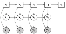
Figure 1: The dynamic Bayesian network for a switching linear dynamical system with four ob-servations. Square nodes denote discrete, and ovals denote continuous random variables. Shading emphasizes that a particular variable is observed.

the assumption that a system cannot restore from a prefault state to a normal state results in a considerable simplification, since many of these components have zero weight.

In Section 3 we review how this sparsity can be exploited in an inference algorithm. As the basis for an EM algorithm it can then straightforwardly be used to compute MAP estimates for the model parameters. The exact inference algorithm has running timeO(T2). Hence for relatively short sequences the constrained transition model makes exact inference feasible. However for larger sequences the exact inference algorithm will be inappropriate. In Section 5 we introduce a flexible class of approximations which can be interpreted as a generalization of expectation propagation (Minka, 2001). It has running timeO(Tκ), with 0≤κ≤_T−2

2

, an integer parameter that can be set according to the available computational resources. Withκ=0 the approximation is equivalent to an iterated version (Heskes and Zoeter, 2002; Zoeter and Heskes, 2005) of generalized pseudo Bayes

2 (Bar-Shalom and Li, 1993) with κ=_T−2

2

exact inference is recovered. Section 6 discusses experiments with inference and MAP parameter estimation on synthetic data and a change point problem in EMG analysis.

2. Benefits of the Constrained Regime Transition Probabilities

An interesting aspect of the model introduced in Section 1 is that, by the restriction in the regime transitions, the number of possible regimes histories is considerably less than the 2T possible histo-ries which would be implied by a system with unconstrained transitions (see e.g. Cemgil et al., 2004; Fearnhead, 2003). If the absorbing state sT+1is not observed, there are T possible regime histories

in the current model. One normal sequence s1:T=n, and T−1 fault sequences: s1:τ=n,sτ+1:T =p,

with 1≤τ≤T−1. In the remainder of this paper we letτdenote the time-slice up to and includ-ing which the regime has been normal, i.e. withτ=T the entire sequence was normal. Under our

assumptions, a fault has to be preceded by at least one prefault state, so if sT+1is observed to be a

fault the entirely normal sequence gets zero weight. So with sT+1observed to be a fault the number

of the possible histories is T−1. If sT+1is observed to be a stop, then only the normal sequence

has nonzero probability.

If the parameters in the model,θ, are known, the exact posterior over a continuous state

p(xt|y1:T,sT+1=f,θ)

computed in a slightly faster way by computing shared partial results only once. This algorithm is introduced in Section 3, and will form a suitable basis for the approximate algorithm from Sec-tion 5. Although we do not expect exact inference to be practical for large T , we can compare approximations with exact results for larger examples than in the regular SLDS case.

The restriction that there are only two non-absorbing regimes is only made for clarity of the exposition. In general the model has M non-absorbing regimes that form stages. No stage can be skipped, and once the system has advanced to the new stage it cannot recover to a previous one. The number of regime histories with non-zero probability in such a system is less than or equal to

TM−1. This can be seen by a simple inductive argument: if M=1 there is only one possible history. If M>1 there are T−(M−1) +1<T possible starting points for the M-th regime (including the

starting point T+1, i.e. when regime M does not occur). The M−1 steps are deducted since the system needs at least M−1 steps to reach the M-th regime. Once the start of the M-th regime is fixed, we have a smaller problem with M−1 regimes of length at most T . So the number of distinct regime histories is bounded by T×TM−2. In principle this is still polynomial in T and for small

M and limited T exact posteriors could be computed, but obviously the need for approximations is

stronger with complexer models.

3. Inference

In this section we will introduce the exact recursive inference algorithm as a special case of the

sum-product algorithm (Kschischang et al., 2001). At this point we assumeθknown, leaving the MAP estimation problem to Section 4.

We are interested in one-slice and two-slice posteriors, p(st,xt|y1:T,θ)and p(st−1,t,xt−1,t|y1:T,θ)

respectively.

By defining ut≡ {st,xt}we obtain a model that has the same conditional independence structure

as the linear dynamical system and the HMM. From time to time we will use a sum notation to denote both the summation over the domain of the discrete variables, and the integration over the domain of the continuous variables in ut. The computational complexity in the current case is due

to the parametric form of the (conditional) distributions over ut as discussed in Section 1.

Assumingθand y1:T fixed and given, the joint probability distribution over all the variables in

the model can be written as a product of factors

p(s1:T+1,x1:T,y1:T|θ) = T+1

∏

t=1

ψt(ut−1,t),

with

ψ1(u1) ≡ p(s1|θ)p(x1|s1,θ)p(y1|x1,s1,θ),

ψt(ut−1,t) ≡ p(st|st−1,θ)p(xt|xt−1,st,θ)p(yt|xt,st,θ) for t=2, . . . ,T , (1)

ψT+1(sT,T+1) ≡ p(sT+1|sT,θ),

and u0≡/0and uT+1≡sT+1. The factor graph (Kschischang et al., 2001) implied by this choice of

factors is shown in Figure 2. Note that we have simplified the figure by not showing the observations

y1:T. These are always observed and are incorporated in the factors.

com-o α1 // u1

α1 _//

β1

o

o o

α2 _//

β1

o

o u2

α2 _//

β2

o

o o

α3 _//

β2

o

o u3

α3 _//

β3

o

o o

α4 _//

β3

o

o u4

α4 _//

β4

o

o o

α5 _//

β4

o

o s5

β5

o

o

ψ1 ψ2 ψ3 ψ4 ψ5

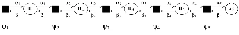
Figure 2: The factor graph corresponding to the change point model and message passing scheme for a model with four observations.

plexity of this algorithm is due to the conditional Gaussian factors and the implied increase in the complexity of the messages.

Algorithm 1 The sum-product algorithm for the SLDS

Forward pass Start the recursion with

p(u1|y1,θ)≡α1(u1) =

ψ1(u1) Z1

, Z1=

∑

u1

ψ1(u1).

For t=1, . . .T

p(ut|y1:t,θ)≡αt(ut) =

∑ut−1αt−1(ut−1)ψt(ut−1,t) Zt|t−1

,

with p(yt|y1:t−1,θ)≡Zt|t−1=∑ut−1,tαt−1(ut−1)ψt(ut−1,t).

Backward pass If sT+1is not observed, start the recursion with

βT(uT) =1.

If sT+1is observed the definition ofβT(uT)is changed accordingly: if sT+1=n, thenβT(sT=

p) =0. Similarly if sT+1=p thenβT(sT=n) =0.

For t=T−1,T−2, . . .1

p(yt+1:T|ut,θ) p(yt+1:T|y1:t,θ)

≡βt(ut) =

∑ut+1ψt+1(ut,t+1)βt+1(ut+1)

∏T

v=t+1Zv|v−1

.

After a forward-backward pass, single-slice and two-slice posteriors are given by

p(ut|y1:T,θ) = αt(ut)βt(ut) p(ut−1,t|y1:T,θ) =

1

Zt|t−1

αt−1(ut−1)ψt(ut−1,t)βt(ut).

In the forward pass the messageαt(ut)≡p(xt,st|y1:t,θ)is not conditional Gaussian, but a

mix-ture of Gaussians conditioned on the regime indicator st. It has t components in total: conditioned

on st =p the posterior p(xt|st =p,y1:t,θ) is a mixture of Gaussians with t−1 components: each

component corresponds to a possible starting point of the prefault regime.

In the smoothing pass an analogous growth of the number of components in the backward messagesβt(ut) occurs, but now growing backwards in time. The single-slice posterior, which is

obtained from the product of the forward and backward messages, has T components for all t. Note that the linear complexity in T is special for the change point model with the restricted regime transitions. In general the number of components in the posterior would grow exponentially.

4. MAP Parameter Estimation

In Section 3 we have assumed that the model parametersθwere known. If they are not known, the expectation-maximization (EM) algorithm (Dempster et al., 1977) with Algorithm 1 in the expecta-tion step, can be used to find maximum likelihood (ML) or maximum a posteriori (MAP) parameter settings. Appendix B lists the M-step updates for the change point model. Appendix C discusses sensible priors on the transition probabilities inΠ.

The learning setting is semi supervised. We assume we are given a set of V training sequences

n

y(_1:Tv)_v

oV

v=1 and that for some, possibly all, we observe s

(v)

T+1. All sequences v for which s

(v)

T+1=s

can be used to estimate the parameters of the normal regime. If s(_Tv₊)₁=f or not observed, the change point from the normal to the prefault regime is inferred in the E-step. The updates from Appendix B then boil down to weighted variants of the linear dynamical system M-step updates, where the weights correspond to the posterior probabilities of being in a particular regime.

The EM algorithm is guaranteed to converge to a local maximum of the likelihood/parame-ter posterior. Different initial parameter estimatesθ(0)may lead the algorithm to converge to different local maxima. This is a known property of the EM algorithm for fitting a mixture of Gaussians. In the current model it can be hoped that the dependence on initialization is less than in the general mixtures of Gaussian case. If there are sequences that are known to be entirely normal (when

sT+1=s) these sequences are only used to determine the characteristics of the normal regime.

Also, due to the change point restriction, some ambiguity is resolved since it is known that the normal precedes the prefault regime.

5. Approximate Inference: Kikuchi Free Energies with Weak Consistency Constraints

The exact inference algorithm presented in Section 3 has the same form as the HMM and Kalman filter algorithms. The messages that are sent,αt(ut)andβt(ut), are not in the conditional Gaussian

family, but are conditional mixtures. As was discussed in Section 3, the number of components in the mixtures grows linear with t and T−t respectively.

A symmetric approximation for the backward pass working directly on theβt(ut) = _pp₍(_yy_tt₊+_1:T1:T_|y|u_1:tt,θ)_,θ)

messages cannot be formulated, since in contrast to theαmessages, theβmessages in general will not be proper distributions and hence a KL divergence is not defined.

This has led to other approaches that introduced additional approximations beyond the pro-jection onto the conditional Gaussian family, (e.g. Shumway and Stoffer, 1991; Kim, 1994). The expectation propagation (EP) framework of Minka (2001) is very suited for this particular model and essentially formulates a backward pass symmetric to the approach outlined above (Zoeter and Heskes, 2005). There are at least two ways of looking at EP. In the first, EP is seen as an iteration scheme where at every step an exact model potential is added to the approximation followed by a projection onto a chosen approximating family. In the second, EP is derived from a particular variational problem. The EP algorithm is introduced in Section 5.2 using the second point of view, which facilitates the description of our generalization in Section 5.3. For a presentation of EP as an iteration of projections the reader is referred to Minka (2001).

The approximate filter and the EP algorithm share that they are greedy: the approximations are made locally. In the EP algorithm the local approximations are made as consistent as possible by iteration. There is no guarantee that the resulting means and covariances in the conditional Gaussian families equal the means and covariances of the exact posteriors. The strong junction tree framework of Lauritzen (1992) operates on trees with larger cliques and approximates messages on a global level. Thereby it does guarantee exactness of means and covariances. For the SLDS a strong junction tree has at least one cluster that effectively contains all discrete variables.

Section 5.3 introduces a generalization of the EP algorithm from Section 5.2. In the general-ization, an extra integer parameterκis introduced that allows a trade-off between computation time and accuracy. The EP algorithm from Zoeter and Heskes (2005) and the strong junction tree from Lauritzen (1992) are then on both extremes.

5.1 Exact Inference as an Energy Minimization Procedure

To facilitate the introduction of the expectation and the generalized expectation propagation al-gorithms, exact inference is introduced in this Section as a minimization procedure. Expectation propagation will follow from an approximation of the objective.

We start by following the variational approach (e.g. Jaakkola, 2001) and turn the computation of−log Z≡ −log p(y1:T|θ)into an optimization problem:

−log Z = min

˜

p [−log Z+KL(p˜(u1:T)||p(u1:T|y1:T,θ))] (2) = min

˜ p

"

−log Z+

∑

u1:T

˜

p(u1:T)log

˜

p(u1:T) Z−1_∏T

t=1ψt(ut−1,t)

#

(3)

= min

˜ p

"

− T

∑

t=1u

∑

p(ut−1,t)logψt(ut−1,t) +

∑

u1:T

˜

p(u1:T)log ˜p(u1:T)

#

. (4)

In (2)–(4) the minimization is over all valid distributions ˜p(u1:T)on the domain u1:T. The KL term

in (2) is guaranteed to be positive and equals zero if and only if ˜p(u1:T) =p(u1:T|y1:T,θ)(Gibbs

In terms of ut the exact posterior factors as

p(u1:T|y1:T,θ) =∏ T

t=2p(ut−1,t|y1:T,θ)

∏T−1

t=2 p(ut|y1:T,θ)

, (5)

so we can restrict the minimization in (4) to be over all valid distributions of the form (5):

−log Z = min {p˜t,q˜t}

"

− T

∑

t=2u

∑

pt(ut−1,t)logψt(ut−1,t)

+ T

∑

t=2u

∑

pt(ut−1,t)log ˜pt(ut−1,t)− T−1

∑

t=2

∑

qt(ut)log ˜qt(ut)

#

. (6)

The minimization is now with respect to one-slice beliefs ˜qt(ut) and two-slice beliefs ˜pt(ut−1,t)

under the constraints that these beliefs are properly normalized and consistent:

˜

pt(ut) =q˜t(ut) =p˜t+1(ut). (7)

To emphasize that the above constraints are exact, and to distinguish them from the weak consistency

constraints that will be introduced below, we will refer to (7) as strong consistency constraints.

Minimizing the objective in (6) under normalization and strong consistency constraints (7) gives exact one- and two-slice posteriors. Since they are exact, the one-slice beliefs ˜qt(ut) will have T

components in our change point model and MT components in a general SLDS.

5.2 Expectation Propagation

As we have seen in the previous section, exact inference inference can be interpreted as a minimiza-tion procedure under constraints. At the minimum, the variaminimiza-tional parameters ˜qt(ut)are equal to the

exact single node marginals. Since these marginals have many components (T in our changepoint model, MT in a general SLDS) even storing the results is computationally demanding.

To obtain an approximation the variational parameters ˜qt(ut) are restricted to be conditional

Gaussian. Recall that ut≡ {st,xt}, so that the conditional Gaussian restriction implies that for every

possible value for st, xt follows a Gaussian distribution, instead of a mixture of Gaussians with a

mixture component for every possible regime history for s1:t−1,t+1:T. This restriction is analogous

to the approximation in the generalized pseudo Bayes 2 (GPB 2) filter (Bar-Shalom and Li, 1993) where in every time update step mixtures of Gaussians are collapsed onto single Gaussians. In fact, as we will see shortly, GPB2 can be seen as a first forward pass in the algorithm that follows from our current approach.

The conditional Gaussian form of Ψt(ut−1,t) and the conditional Gaussian choice for ˜qt(ut)

imply that at the minimum in (6) ˜pt(ut−1,t)is conditionally Gaussian as well (see Appendix D).

If we restrict the form of ˜qt(ut), but leave the consistency constraints exact as in (7), a minimum

of the free energy has a very restricted form. The strong consistency constraints would imply that the two exact marginals ∑ut−1p˜t(ut−1,t) =p˜t(ut) and ∑utp˜t(ut−1,t) =p˜t−1(ut−1) are conditional Gaussians instead of conditional mixtures. This holds only if the continuous variables xt−1,t are

independent of the discrete states st−1,t in ˜pt(ut−1,t).

To obtain non-trivial approximations, the single-slice beliefs ˜qt(ut) are restricted to be

of having equal marginals we only require overlapping beliefs to be consistent on their overlapping expectations

hf(ut)ip˜t =hf(ut)iq˜t =hf(ut)ip˜t+1 , (8)

where f(ut)is the vector of sufficient statistics of the conditional Gaussian family over ut as defined

in Appendix A.

With these restrictions ˜qt(ut)is in general not the marginal of ˜pt(ut−1,t), so one-slice and

two-slice beliefs satisfying (8) do not lead to a proper distribution of the form (5). As a result, although we started the derivation with the variational (mean-field) bound (2), the objective we aim to mini-mize is not guaranteed to be a bound on−log Z.

The EP algorithm can be seen as fixed point iteration in the dual space of the constrained minimization problem (Zoeter and Heskes, 2005, Appendix D). This is in direct analogy to the interpretation of loopy belief propagation as fixed point iteration in the dual space of the Bethe free energy (Yedidia et al., 2005).

Algorithm 2 presents the generalization that will be derived next, but withκ=0 it gives the basic update equations of this section. In a first forward pass, with all backward messages initialized as

βt(ut) =1 (i.e. effectively with no backward messages), the updates are equivalent to the greedy

projection filter GPB2.

As a final note we remark that this approximation, and even the update scheme, can also be derived from the iterative projection point of view of EP. To obtain Algorithm 2 withκ=0, the ap-proximating family should be chosen to be a product of independent conditional Gaussians (Zoeter and Heskes, 2005).

5.3 Generalized Expectation Propagation

Since we have associated the EP approach to an approximation of the Bethe free energy (6), we can extend the approximation analogously to Kikuchi’s extension of the Bethe free energy (Yedidia et al., 2005).

In the EP free energy (6) the minimization is w.r.t. beliefs over outer clusters, ˜pt(ut−1,t), and

their overlaps, ˜qt(ut−1,t). In the so-called negative entropy, T

∑

t=2u

∑

pt(ut−1,t)log ˜pt(ut−1,t)− T−1

∑

t=2

∑

qt(ut)log ˜qt(ut),

from (6), the outer clusters enter with a plus, the overlaps with a minus sign. These 1 and -1 factors can be interpreted as counting numbers that ensure that every variable effectively is counted once in the (approximate) entropy in (6). If the free energy is exact (i.e. no parametric choice for the beliefs, and strong consistency constraints), the local beliefs are exact marginals, and as in (5), the counting numbers can be interpreted as powers that dictate how to construct a global distribution from the marginals.

In Kikuchi’s extension the outer clusters are taken larger. The minimization is then w.r.t. beliefs over outer clusters, their direct overlaps, the overlaps of the overlaps, etc. With each belief again proper counting numbers are associated.

One way to construct a valid Kikuchi based approximation is as follows (Yedidia et al., 2005). Choose outer clusters uouter(i)and associate with them the counting number couter(i)=1. The outer

s1 / /

s2 //

s3 //

s4 //

s5 //

. . . //_sT

/

/sT+1

x1

/

/x2 //

x3 //

x4 //

x5 //

. . . //xT

y1 y2 y3 y4 y5 . . . yT

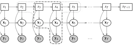
Figure 3: Cluster definitions forκ=0 (dashed) andκ=1 (dotted).

in at least one outer cluster. Then recursively define the overlaps of the outer clusters u_over(i), the overlaps of the overlaps, etc. The counting number associated with clusterγis given by the M ¨obius recursion

c_γ=1−

∑

u_γ0⊃uγ

c_γ0 . (9)

A crucial observation for the SLDS is that it makes sense to take outer clusters larger than the cliques of a (weak) junction tree. If we do not restrict the parametric form of ˜qt(ut)and keep exact

constraints, the cluster choice in (5) gives exact results. However, the restriction that ˜qt(ut)must be

conditional Gaussian, and the weak consistency constraints imply an approximation: only part of the information from the past can be passed on to the future and vice versa. With weak constraints it is beneficial to take larger outer clusters and larger overlaps, since the weak consistency constraints are then over a larger set of sufficient statistics and hence “stronger”.

We define symmetric extensions of the outer clusters as depicted in Figure 3. The size of the clusters is indicated by 0≤κ≤_T−2

2

:

u_outer(i) =

s_{i:i+2(κ+1)−1},xi+κ,i+κ+1 , for i>1∧i<T−2τ+2 (10) uover(i) = uouter(i)∩uouter(i+1). (11)

In the outer clusters only the discrete space is extended because the continuous part can be integrated out analytically and the result stays in the conditional Gaussian family. The first and the last outer cluster have a slightly larger set. In addition to the set (10) the first cluster also contains x1:i+κ−1

and the last also xi+κ+2:T. This implies a choice where the number of outer clusters is as small as

possible at the cost of a larger continuous part in the first and the last cluster. A slightly different choice would have more clusters, but only two continuous variables in every outer cluster.

To demonstrate the construction of clusters and the computation of their associated counting numbers we will look at the case ofκ=1. Below the clusters are shown schematically, with outer clusters on the top row, and recursively the overlaps of overlaps, etc.

s1,2,3,4 x1,2,3

s2,3,4,5 x3,4

s3,4,5,6 x4,5

s4,5,6,7 x5,6,7 s2,3,4

x3

s3,4,5 x4

s4,5,6 x5 s3,4 s4,5

s4

The overlaps of overlaps have five clusters in which they are contained, their counting numbers are 1−(3−2) =0. The clusters on the lowest level have nine parents, which results in a counting number 1−(4−3+0) =0. It is easily verified that withκ=0 we obtain the cluster and counting number choice of Section 5.2.

A second crucial observation for the SLDS is that the choice of outer clusters (10) implies that we only have to consider outer clusters and direct overlaps, i.e. the phenomenon that all clusters beyond the direct overlaps get an associated counting number of 0 in the example above extends to allκ. This is a direct result of the fact that the clusters from (10) form the cliques and separators in a (weak) junction tree. I.e. another way to motivate a generalization with the cluster choice (10) is to replace (5) with

p(u1:T|y1:T,θ) =

∏N

i=1p(uouter(i)|y1:T,θ)

∏N−1

j=1 p(uover(j)|y1:T,θ)

, (12)

and use this choice in (4) to obtain an extension of (6). In (12), N=T−2κ−1 denotes the number of outer clusters in the approximation.

The aim then becomes to minimize

FGEP = −

N

∑

i=1uouter

∑

pi(uouter(i))logΨ(i)(uouter(i))

+ N

∑

i=1uouter

∑

pi(uouter(i))log ˜pi(uouter(i))

− N−1

∑

i=1uover

∑

qi(uover(i))log ˜qi(uover(i)), (13)

w.r.t. the potentials ˜pi(uouter(i)), and ˜qi(uover(i)). For i=2,3, . . .N−1, the potentialsΨ(i)(uover(i))

are identical to the potentialsψi+κ+1(ui+κ,i+κ+1)from (1). At the boundaries they are a product of

potentials that are “left over”:

Ψ(1) ₌ κ+

∏

j=1

ψj(uj−1,j)

Ψ(N) ₌

∏

j=T−κ

ψj(uj−1,j),

withΨ(1)=∏T

j=1ψj(uj−1,j)if N=1.

The approximation in the generalized EP free energy, FGEP, arises from the restriction that

˜

qi(uover(i))is conditional Gaussian and from the fact that overlapping potentials are only required to

be weakly consistent

f(uover(i))

˜ pi=

f(uover(i))

˜ qi =

f(uover(i))

˜ pi+1 .

enforce the weak consistency constraints. Just as for EP itself, convergence of Algorithm 2 is not guaranteed.

In Algorithm 2 the messages are initialized as conditional Gaussian potentials, such that

˜

q(uover(i)) =αi(uover(i))βi(uover(i))

are normalized. A straightforward initialization would be to initialize all messages with 1. If at the start all products of matching messages are normalized, we can interpret the product of local normalizations∏N_i=1Zias an approximation of the normalization constant Z.

Algorithm 2 Generalized EP for an SLDS

Compute a forward pass by performing the following steps for i=1,2, . . . ,N−1, with i0≡i, and a

backward pass by performing the same steps for i=N,N−1, . . . ,2, with i0≡i−1. Iterate forward-backward passes until convergence. At the boundaries keepα0=βN =1.

1. Construct an outer-cluster belief,

˜

pi(uouter(i)) =

αi−1(uover(i−1))Ψ(i)(uouter(i))βi(uover(i))

Zi

,

with Zi=∑uouter(i)αi−1(uover(i−1))Ψ (i)_(u

outer(i))βi(uover(i)).

2. Marginalize to obtain a one-slice marginal

˜

pi(uover(i0₎) =

∑

uouter(i)\uover(i0) ˜

pi(uouter(i)).

3. Find ˜qi0(u_over(i0₎)that approximates ˜p_i(u_over(i0₎)best in Kullback-Leibler (KL) sense:

˜

qi0(u_over(i0₎) =Collapse ˜p_i(u_over(i0₎) .

4. Infer the new message by division.

αi(uover(i)) =

˜

qi(uover(i)) βi(uover(i))

, βi−1(uover(i−1)) =

˜

qt−1(uover(i−1)) αi−1(uover(i−1))

.

Figure 4 gives a graphical representation of Algorithm 2 for κ=0. Figure 5 gives a similar schema forκ=1. The two figures show what information is lost when the one-slice beliefs are collapsed.

The choice of 0≤κ≤_T−2

2

now allows a trade off between computational complexity and degrees of freedom in the approximation. Withκ=0, we obtain the EP/Bethe free energy equiv-alent to Zoeter and Heskes (2005). With κ=_T−2

2

there is only one cluster and we obtain a

s2 s2s3 s3 s2s3 s2s3 s3

α1 Ψ(2) β2 p˜2 p˜2 q˜2

∑

s2,x2 Col. =

× × ×

× ×

×

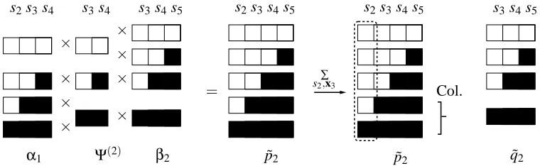
Figure 4: A schematic representation of steps 1, 2 and 3 from Algorithm 2 withκ=0, for a se-quence with more than 3 observations. The potentialΨ(2)(u2,3)contains three Gaussian

components: p(y3,x3|x2,s2=n,s3=n), p(y3,x3|x2,s2=n,s3=p), and p(y3,x3|x2,s2=

p,s3=p). The(p,n)assignment gets zero weight by the non-recovery assumption and is

therefore not shown. Combinations with absorbing states are excluded since the sequence does not stop at 3. Every component is encoded by a row, with white squares denoting normal, and black squares prefault regimes. The messagesα1(x2,s2) andβ2(x3,s3)are

conditional Gaussian by construction and hence each have two components: one corre-sponding to normal and one to prefault. Exact marginalization gives ˜p2(x3,s3), which

still consists of three components. To emphasize that s2 is not part of the domain, it is

enclosed by a dashed rectangle. Conditioned on s3=p, ˜p2(x3|s3=p)is a mixture. This

mixture is collapsed to obtain a conditional Gaussian approximation ˜q2(u3).

PSfrag replacements

s2s3s4 s3s4 s3s4s5 s2s3s4s5 s2s3s4s5 s3s4s5 s6

α1 Ψ(2) β2 p˜2 p˜2 q˜2

∑

s2,x3

Col.

= ×

× ×

×

× ×

× ×

to be extremely likely. In fact, we have not seen the performance degrade with largerκin any of our experiments.

6. Experiments

In Section 6.1 we explore the properties of the learning algorithm and approximate inference in a controled setting with artificial data. Section 6.2 presents experiments with EMG data.

6.1 Synthetic Data

As discussed in Section 4 the constraints in the regime transitions aid in learning. When a stop is observed in the trainset, the entire sequence is guaranteed to be normal. Also, the fact that the normal regime precedes the prefault regime resolves the invariance under relabeling that would be present in a general switching linear dynamical systems setting. Experiments with artificially generated data shows that even with a relatively small trainset the two regimes can be learned fairly reliably.

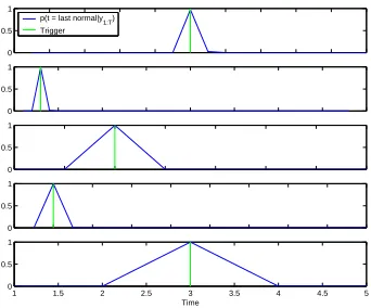
We ran experiments where 15 train and 5 test sequences were generated from randomly drawn change point models. The classes of the train sequences (stop or fault) were observed, the classes of the test sequences were unknown. Figure 6 is not an a-typical result. In many experiments we find that both the classification (determining whether the sequence ended in a stop or in a fault) and the determination of the change point were often (near) perfect.

The MAP

τmap=argmax

τ p(s1:τ=n,sτ+1:T =p|y1:T,θML),

is taken as the predicted change point. In 10 replications the mean squared error between the actual and the inferred change point was 6.6 (standard deviation 11.75, median 0).

These results are encouraging, but may also be largely due to the fact that arbitrarily drawn models may not pose a serious challenge. Qualitatively the replicated experiments show that for most replications the errors are close to 0 (as in Figure 6). This explains the low median. In a few replications the model has learned normal and prefault classes that are different from the true generating model and hence result in large errors. In these replications we still see the “arbitrariness” of the fitted clusters that is common to the mixtures of Gaussians learning. We do not investigate a proper characterization of “difficult” and “easy” models here, but discuss some of the possible pitfalls with the approach in Section 6.2.

To explore the properties of the approximations developed in Section 5, we ran 10 experiments where a single sequence of length 10 was generated from a randomly drawn model. For every sequence, approximate single node posteriors ˜q(xt|y1:T,θ)were computed using Algorithm 2 with

κ=0,1,2,3,4. Figure 7 shows the maximum absolute error in the single node posterior means as a function ofκ. The lines show the average over the 10 experiments, the maximum encountered, and the minimum. For sequences with length 10,κ=4 is guaranteed to give exact results. So in theory, the lines in Figure 7 should meet atκ=4. The discrepancies in Figure 7 are explained by different round off errors in our implementations of Algorithm 2 and the strong junction tree.

0 0.5 1

p(t = last normal|y

1:T)

Trigger

0 0.5 1

0 0.5 1

0 0.5 1

1 1.5 2 2.5 3 3.5 4 4.5 5

0 0.5 1

Time

Figure 6: Shown are the inferred and true change points on 5 test sequences. The EM algorithm from Section 4 was presented with 15 artificially generated train sequences, all of which resulted in an observed fault.

0 1 2 3 4

10−20 10−15 10−10 10−5 100

MAD on single−node posterior mean

κ

Maximum Absolute Deviation

Mean Max Min

6.2 Detecting Changes in EMG Signals

The algorithm from Section 4 was used to detect changes in EMG patterns in the stumbling experi-ments from Schillings et al. (1996).

In Schillings et al. (1996) bipolar electromyography (EMG) activity in human subjects were recorded. The subjects were walking on a treadmill at 4 km/h. By releasing an object suspended from an electromagnet the subjects could be tripped at a specified phase in the walking pattern. Partially obscured glasses and earplugs ensured that the tripping was unexpected.

In the experiments video recordings and a pressure-sensitive strip attached to the obstacle sig-naled the tripping onset. We extracted an interesting change point problem from this experiment by only looking at the EMG signals measured at the biceps femoris at the contra lateral side, i.e. by only looking at a signal which is indicative of the activity of the large muscle in the upper leg at the non-obstructed side.

In our experiments we used data for a single subject. The dataset consisted of 15 control trials where no object was released and 8 stumbling experiments. All sequences were of equal length, and started roughly at the same phase in the walking pattern. The control trials were treated as normal sequences and the 8 others as fault sequences. In the first experiments the class of the sequences were assumed to be known and the aim for the algorithm was to determine the change points.

The original series were raised to a power of -.2 to obtain signals that seemed in agreement with the additive noise assumptions. The initial parameter settings for the normal regime was in Fourier

form (West and Harrison, 1997). The chosen harmonic components were obtained from a discrete

Fourier transform. Based on the residuals of the 15 normal sequences a model with 4 harmonics was selected.

There were three different phases of training. In the first, only the normal sequences were considered and the transition matrix Anwas kept fixed. In the second phase, again only the normal

regime was considered, but Anwas also fitted. In all phases of learningκwas set to 50, i.e. inference

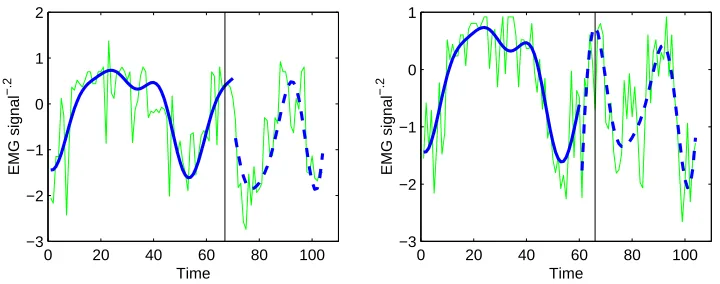
results were indistinguishable from exact. The result of the first two phases is characterized by the left plot in Figure 8. In the third phase all parameters were fitted. The prefault model was initialized as an outlier model, i.e. the parameters for the prefault regime were copies of the normal regime, but the noise covariances were larger. The characteristics of the entire model are depicted in the right plot of Figure 8.

After convergence, the mean absolute distance between the MAP change point and the triggers in the 8 fault sequences is 4.25, with standard deviation 1.49. Figure 9 shows the posteriors p(s1:t=

n,st+1:T =p|y1:T,θ)and the trigger signals for the 8 fault sequences. There are two typical errors:

0 20 40 60 80 100 −3

−2 −1 0 1 2 3

Time

EMG signal

−.2

0 20 40 60 80 100

−3 −2 −1 0 1 2

Time

EMG signal

−.2

Figure 8: Characteristics of the learned model. The left plot shows the transformed EMG signals for all normal sequences in thin solid lines. The thick solid line shows the model prediction with the regime indicators clamped to normal. The right plot shows all EMG signals from stumbling trials. The light thick line shows model predictions with all regime indicators clamped to normal just as in the left plot. The dark thick line shows the model predictions with the regime indicators clamped to normal from 1 to 70 and to prefault from 71 to 104. This change point was hand picked and roughly coincides with the average trigger time.

0 0.5 1

p(t = last normal|y_1:T) Trigger

0 0.5 1

0 0.5 1

0 0.5 1

0 0.5 1

0 0.5 1

0 0.5 1

0 20 40 60 80 100 120

0 0.5 1

Time

Figure 9: Stumble detection based on a single EMG signal. Vertical bars show the true stumbling trigger. The solid curves show the posterior probability that t was the last normal time point.

the model such that the expected muscle activity is continuous even during a change point might resolve some of the observed overfitting.

0 20 40 60 80 100 −3

−2 −1 0 1 2

Time

EMG signal

−.2

0 20 40 60 80 100

−3 −2 −1 0 1

Time

EMG signal

−.2

Figure 10: Thin lines show the EMG recordings of a single sequence. The vertical bars show the moment at which the stumble was triggered. The thick lines give an indication of the learned models. They were constructed by clamping the discrete states of the model to the MAP change point value and computing the predicted mean EMG signal (light lines represent the normal, dark lines the prefault regime). The left plot shows the second (from the top) sequence from Figure 9 and gives an acceptable detection of the prefault regime. The right plot shows the third sequence and represents a typical overfit: the model uses its degrees of freedom to fit outliers preceding the change point in some of the sequences. This explains the too early warnings in Figure 9.

which p(s1:T =n|y1:T,θ)≥.5 was classified as normal. With this scheme all abnormal sequences,

and 13 out of 15 normal sequences were correctly classified.

7. Discussion

Motivated by fault and change detection problems in dynamical systems we have introduced a switching linear dynamical system with constrained regime transition probabilities. The system is assumed to start in a normal regime and to either result in an absorbing stop state or change to a prefault regime. Once the system reaches a prefault regime, it cannot recover and eventually has to result in a fault.

These model assumptions have several advantages. As discussed in Sections 2 and 3, the as-sumption that the system cannot recover can be exploited to yield an algorithm that computes exact state and regime posteriors in time polynomial in the number of observations.

Since the number of observations, T , may grow very large we have introduced an approximate inference algorithm in Section 5.

The algorithm, generalized expectation propagation (GEP), can be derived as a fixed point itera-tion that aims to minimize a variant of a Kikuchi free energy. One way of interpreting the algorithm is that it sends messages along a weak junction tree as if it was a strong junction tree. This is anal-ogous to the interpretation of loopy belief propagation as an algorithm that sends messages on a loopy graph as if it was operating on a tree.

The change point model has two pleasant properties that makes the application of GEP particu-larly elegant. The first is the fact that the conditional independencies in the underlying model form a chain. Therefore we can straightforwardly choose outer clusters in the Kikuchi approximation such that they form a (weak) junction tree. We have shown that the resulting GEP updates then simplify since only outer clusters and direct overlaps need to be considered, i.e. from an implemen-tation point of view the algorithm is not more complicated than the ordinary EP algorithm. Also, since there are no loops disregarded, increasing the cluster size leads to relatively “well behaved” approximations; they satisfy the perfect correlation and non-singularity conditions from Welling et al. (2005). Increasing the size of the clusters in our approximation implies that more statistics are passed from past to future and vice versa. This makes an improvement in the approximation very likely (although an improvement is only guaranteed forκ ∝T at which point it becomes

ex-act). This is in contrast to the generalization of belief propagation on e.g. complete graphs, which is notorious for the fact that with unfortunate choices of clusters the quality degrades with larger clusters (Kappen and Wiegerinck, 2002). In our experiments with the change point model, we have never observed a degradation of the quality with an increase ofκ. This suggests thatκshould be set as large as computing power permits.

The first pleasant property of the change point model leads to the observation that in approxi-mations with weak consistency constraints it makes sense to take clusters larger than is necessary to form a (weak) junction tree. This property is shared with all models that have (weak) junction trees with reasonable cluster sizes, in particular chains and trees.

The second property is due to the no-recovery assumption property in the change point model. This implies that exact inference is polynomial in T , and also that approximate inference is poly-nomial inκ, which makes a wide range ofκ’s feasible. In a general SLDS exact inference scales exponential in T and approximate inference exponential inκ.

Although we did not discuss this in Section 5, the GEP algorithm is not restricted to trees or chains. In models with cycles and complicated parametric families, an algorithm can send messages as if it is sending messages on a strong junction tree, whereas the underlying cluster choices do not form a tree, neither a weak nor a strong one. See Heskes and Zoeter (2003) for a discussion.

Algorithm 2 is conjectured to be a proper generalization of the EP framework. Although tree EP (Minka and Qi, 2004) results in approximations that are related to (variants of) Kikuchi free energies it is unlikely that a tree or another clever choice of the approximating family would result in Algorithm 2. Since the overlapping ˜q(uover(i)) are not strongly consistent they cannot easily be

Acknowledgments

We would like to thank I. Schillings for providing the EMG data that was used in the experiments of Section 6.2.

Appendix A. Operations on Conditional Gaussian Potentials

To allow for simple notation in the main text this appendix introduces the conditional Gaussian (CG) distribution. A discrete variable s and a continuous variable x are jointly CG distributed if the marginal of s is multinomial distributed and, conditioned on s, x is Gaussian distributed. Let x be

d-dimensional and let S be the set of values s can take. In moment form the joint distribution reads

p(s,x) =πs(2π)−d/2|Σs|−1/2exp

−1

2(x−µs) >_Σ−1

s (x−µs)

,

with moment parameters {πs,µ_s,Σs+µsµ>s}, whereπs is positive for all s and satisfies∑sπs=1

andΣsis a positive definite matrix. The definition ofΣs+µsµ>s instead ofΣs is motivated by (16)

below. For compact notation sets with elements dependent on s will implicitly ranges over s∈S. In

canonical form the CG distribution is given by

p(s,x) =exp

gs+x>hs−

1 2x

>_K

sx

, (14)

with canonical parameters{gs,hs,Ks}.

The so-called link function g(.)maps canonical parameters to moment parameters:

g({gs,hs,Ks}) = {πs,µ_s,Σs+µsµ>s}

πs = exp(gs−¯gs) µ_s = K_s−1hs

Σs = Ks−1,

with ¯gs≡1₂log|K_2πs| −₂1h>sKshs, the part of gsthat depends on hsand Ks. The link function is unique

and invertible:

g−1({πs,µ_s,Σs+µsµ>s}) = {gs,hs,Ks} gs = logπs−

1

2log|2πΣs| − 1 2µ

>

sΣ−s1µs hs = Σ−s1µs

Ks = Σ−s1.

A conditional Gaussian potential is a generalization of the above distribution in the sense that it has the same form as in (14) but need not integrate to 1. Ksis restricted to be symmetric, but need

not be positive definite. If Ksis positive definite the moment parameters are determined by g(.).

Multiplication and division of CG potentials are the straightforward extensions of the analogous operations for multinomial and Gaussian potentials. In canonical form:

φ(s,x;{gs,hs,Ks})φ(s,x;{g0_s,h0_s,K_s0}) = φ(s,x;{gs+g0s,hs+h0s,Ks+Ks0})

φ(s,x;{gs,hs,Ks})/φ(s,x;{g0_s,h0_s,K_s0}) = φ(s,x;{gs−g0s,hs−h0s,Ks−Ks0}).

With the above definition of multiplication we can define a unit potential

1(s,x)≡φ(s,x;{0,0,0}),

which satisfies 1(s,x)p(s,x) = p(s,x) for all CG potentials p(s,x). We will sometimes use the shorthand 1 for the unit potential when its domain is clear from the text.

In a similar spirit we can define multiplication and division of potentials with different domains. If the domain of one of the potentials (the denominator in case of division) forms a subset of the do-main of the other we can extend the smaller to match the larger and perform a regular multiplication or division as defined above. The continuous domain of the small potential is extended by adding zeros in hs and Ksat the corresponding positions. The discrete domain is extended by replicating

parameters, e.g. extending s to[s t]>_{we use parameters g}

st=gs, hst=hs, and Kst=Ks.

Marginalization is less straightforward for CG potentials. Integrating out continuous dimensions is analogous to marginalization in Gaussian potentials and is only defined if the corresponding moment parameters are defined. Marginalization is then defined as converting to moment form, ‘selecting’ the appropriate rows and columns from µ_sandΣs, and converting back to canonical form.

More problematic is the marginalization over discrete dimensions of the CG potential. Summing out s results in a distribution p(x)which is a mixture of Gaussians with mixing weights p(s), i.e. the CG family is not closed under summation. In the text we will sometimes use, somewhat sloppily, the∑notation for both summing out discrete and integrating out continuous dimensions.

We define weak marginalization (Lauritzen, 1992), as exact marginalization followed by a

collapse: a projection of the exact marginal onto the CG family. The projection minimizes the

Kullback-Leibler divergence KL(p||q) between p, the exact (strong) marginal and q, the weak marginal:

q(s,x) = argmin

q∈CG

KL(p||q)

≡ argmin

q∈CG

∑

p(s,x)logp(s,x)

q(s,x) .

This projection has the property that, conditioned on s the weak marginal has the same mean and covariance as the exact marginal. The weak marginal can be computed by moment matching (Whit-taker, 1989). If p(x|s)is a mixture of Gaussians for every s with mixture weightsπr|s, means µsr,

and covariancesΣsr (e.g. the exact marginal∑rp(s,r,x)of CG distribution p(s,r,x)), the moment

matching procedure is defined as

Collapse(p(s,x)) ≡ p(s)N(x; µ_s,Σs) µ_s ≡

∑

r

πr|sµsr

Σs ≡

∑

r

πr|s

Σsr+ (µsr−µs)(µsr−µs)>

Note that this projection, contrary to exact marginalization, is not linear, and hence in general:

Collapse(p(s,x)q(x))=6 Collapse(p(s,x))q(x).

In even more compact notation, with δs,m the Kronecker delta function, we can write a CG

potential as

p(s,x) = exp[ν>f(s,x)], with (15)

f(s,x) ≡ [δs,mδs,mx>δs,mvec(xx>)>|m∈S]>

ν ≡ [gsh>s −

1

2vec(Ks)

>_|s∈S]>

the sufficient statistics, and the canonical parameters respectively. In this notation the moment parameters follow from the canonical parameters as

g(ν) =hf(s,x)i_exp[ν>_f(s,x)]≡

∑

s Z

dx f(s,x)exp[ν>f(s,x)]. (16)

Appendix B. The M-step Updates

We defineθas the set of all parameters

θ≡

Πi→j,m1,V1,Aj,Cj,µj,r2j|(i,j)∈G ,

and G as the set of allowed regime transitions

G≡ {(n,n),(n,p),(n,s),(p,p),(p,f)},

with the shorthands n,p,s,f, for normal, prefault, stop, and fault regimes respectively. For now we assume a flat prior onθ, i.e. we compute ML instead of MAP estimates.

In the M-step we maximize the expected complete data log-likelihood ˆLwith respect toθ. The expected complete data log-likelihood is defined as:

ˆ

L(y1:T,sT+1|θ) ≡ Ep(s1:T,x1:T|y1:T,sT+1,θold)[log p(y1:T,x1:T,s1:T+1|θ)].

Using the conditional independencies implied by the model and the constraints in the regime prior and transitions we can rewrite it as:

ˆ

L(y1:T,sT+1|θ) = p(s1=n|y1:T,sT+1,θold)Ep(x1|s1=n,y1:T,sT+1,θold)logN(x1; m1,V1)

+

∑

(i,j)∈G T+1

∑

t=2

p(st = j,st−1=i|y1:T,sT+1,θold)logΠi→j

+

∑

j∈{n,p}

T

∑

t=2

p(st= j|y1:T,sT+1,θold)

Ep(xt−1,t|st=j,y1:T,sT+1,θold)logN(xt; Ajxt−1,Qj)

+

∑

j∈{n,p}

T

∑

t=1

p(st= j|y1:T,sT+1,θold)

Note that from the model assumptions p(s1=n|y1:T,sT+1,θold) =1.

The M-step updates for the parameters follow by adding Lagrange multipliers for the normal-ization constraints and setting partial derivatives to 0.

We useh·i_·to denote weighted expectations, and pt(i j)as a shorthand for the relevant posterior

e.g.

hf(xt−1,xt)ipt(i j) = p(st−1=i,st =j|y1:T,sT+1,θold)

× Z

dxt−1,tf(xt−1,xt)p(xt−1,t|st−1=i,st = j,y1:T,sT+1,θold).

In this notation h1i_p

t(i j) simply gives a weighting factor. In the statistics above, and hence in the update equations below, we recognize forms similar to a regular LDS but now with a weighting term that would not be present in the non-switching case.

The updates forΠi→j are weighted versions of the standard HMM updates. The prior is

deter-ministic (all sequences start in the normal regime) and fixed. The updates read:

Anew_j = T

∑

t=2

D

xtx>t−1

E

pt(·j)

!

T

∑

t=2

D

xt−1xt>−1

E

pt(·j)

!−1

Qnew_j =

∑T t=2

xtxt>

pt(·j)−A

new j ∑tT=2

xtx>t−1

>

pt(·j)

∑T

t=2h1ipt(·j)

mnew₁ = hx1i_p1(n) V₁new = Dx1x>1

E

p1(n)−m

new

1 (mnew1 )>

Πnew

i→j ∝ T+1

∑

t=2 h1i_p

t(i j) ∀(i,j)∈G.

We compute the new output matrix Cjand the new mean µjjointly by adding µj as an extra column

to Cj and adding an entry to the continuous state that is always 1. We define

Pt,j ≡

xtx>t

hxti hxti> h1i

mt,j ≡

hxti h1i

˜

Cnew_j ≡

Cnew_j µnew_j ,

with the weighted expectationsh·iover pt(j), to arrive at

˜

Cnew_j = T

∑

t=1 ytm>t,j

!

T

∑

t=1 Pt,j

!−1

r2 new_j =

∑T

t=1yt>yth1ipt(j)−tr

˜

Cnew_j >∑T_t=1ytm>t,j

where d is the dimensionality of the observations yt.

When sT+1=f, or if it is not observed, posterior distributions such as p(xt−1,t|st−1=i,st = j,y1:T,sT+1=f,θold)are mixture of Gaussians (the sT+1=s case results in a straightforward LDS

variant). For the updates described above first and second moments of these mixtures are required. They can be computed analytically and simply boil down to the weighted sum of the means and second moments of the individual components. For example, xtxt>−1

pt(·n), is based on a mixture with T−t−1 components (if sT+1is observed to be a fault), each corresponding to a possible end

of the normal regime.

D

xtx>t−1

E

pt(·n)

= T−1

∑

τ=t

D

xtxt>−1

E

pt:τ(·n:n)

≡ T−1

∑

τ=t

p(s1:τ=n|y1:T,sT+1=f,θold) ×

Z

dxt−1,txtx>t−1p(xt−1,t|s1:τ=n,sT+1=f,θold).

If the trainset consists of V sequences instead of one, in the above update steps all sums∑_tb_=aare replaced by∑V_v=1∑bv

t=a. Only the update for m1and V1change. The posterior over x1is a mixture of

Gaussians with one mixture component for every sequence. The required sufficient statistics follow again by a collapse.

Appendix C. Prior Distributions

In practice, if the underlying models for normal and prefault regimes are relatively “far apart”, we expect that the model parameters can be inferred reliably. For example if the prefault regime has an entirely different offset in the observation model, the prefault subsequences lie in an entirely different region of sensor space, which makes it easy to distinguish between the two. However in many practical applications we expect the difference not to be so profound. In this Section we introduce sensible priors on the parameters such that a priori knowledge can be incorporated.

Our main concern is with priors on the regime transition probabilities. There are three free parameters in the transition probabilities model: Πn→n, Πn→p and Πp→p (Πn→s≡1−(Πn→n+

Πn→p), andΠp→f≡1−Πp→pby construction).

The conjugate prior forΠp→pis

p(Πp→p|νp,λp)∝ Πp→p

νpλp

1−Πp→p

νp

.

The parametersνpandλphave a natural interpretation as the number of sequences and the average

number of p→p transitions in a hypothesized set of “pseudo observed” sequences.

A similar reasoning holds for the parameters Πn→n, Πn→s, and Πn→p. Suppose we observe Vns+Vnpsequences with on average ¯ln n→n transitions, and Vnsof these ended in a stop and Vnp

switched to prefault. The probability of observing this set S of sequences is

p(S|Πn→n,Πn→s,Πn→p) = (Πn→n)(Vns+Vnp) ¯ ln_(Π

n→s)Vns Πn→p

Vnp

.

The conjugate prior is

p(Πn→n,Πn→s,Πn→p|νns,νnp,λn)∝(Πn→n)(νns+νnp)λn(Πn→s)νns Πn→p

νnp