2016 3rd International Conference on Information and Communication Technology for Education (ICTE 2016) ISBN: 978-1-60595-372-4
1. INTRODUCTION
Negative selection algorithm is one of the main algorithms of artificial immune system, which has been widely used in different areas [1]. In essence, the negative selection algorithm is a self/non self recognition technique that is inspired by the maturation process of T cells in the thymus: if T cells recognize autologous elements, it will be cleared. The typical negative selection algorithm is composed of two stages. First of all, it is the generation of the detector set, and then uses the detector set to check the new samples. So it can be seen that the quality of the detector directly affects the result of the test. The detector expression method is a binary representation and real valued representation, due to the real valued said is more suitable to describe practical problems, the researchers attention [2] .literature [3] first proposed the real valued negative selection algorithm and the fixed length detector, due to the difficulty in determining the appropriate detector radius. Therefore, detection performance is poor; literature [4] proposed variable length detector generating algorithm, improves the detection rate, and has been widely used in the different of the anomaly detection domain. On the basis of literature [4], different researchers have made different improvement work
[5-9]
. However, almost all of the algorithms are considered as candidate detectors for each individual point as a candidate for the individual and excluded from the detector. This approach may lead to some
deviations, especially in the regions of the self and non self regions of the boundary. The traditional detection rate and false alarm rate are mainly caused by the boundary of self and non self, so the algorithm must consider the performance of the self / non self boundary. This paper calls this problem for the border dilemma.
Based on this, this paper proposes a new algorithm of edge detection. The basic idea of this algorithm is that training data is considered as a whole, and not independent of the point; independent self point cannot be declared a regional is self region, only a set of points together to show that a self region. Based on the VRNSA[4] algorithm, using real valued, using variable length detector. The experimental results show that this algorithm has certain advantages, especially for the case of self / non self boundary element.
2. BOUNDARY PROBLEM OF NEGATIVE SELECTION ALGORITHM
In terms of real valued representation, according to the meaning of self region, a self elements or self elements set specific said what kind of data depends on matching rule [8]. Usually, it can be considered that a region of a circle is normal (self), which is a generalization of the self, which is similar to that of the binary representation. At the same time, it can be considered that only the normal state of the body is normal, and the other is abnormal state. In this
An Improved Detector Set Generation Mechanism in Negative
Selection Algorithm
Bo Hu
Science and Technology College Jiangxi Normal University Nanchang, China
ABSTRACT: in view of the shortcomings of the detector generation mechanism in the existing negative selection algorithm, a new method of boundary detection is proposed to deal with the problem of the boundary dilemma. In the algorithm, it is used as the self region of the body and its adjacent points. The realization process and advantages of the algorithm are given. The algorithm is validated by the synthetic data set 2DSyntheticData and the actual Iris data set and the Biomedical data set. Experimental results show that the detection rate of this algorithm is high, especially the points that are in the self and non self boundary can be detected effectively.
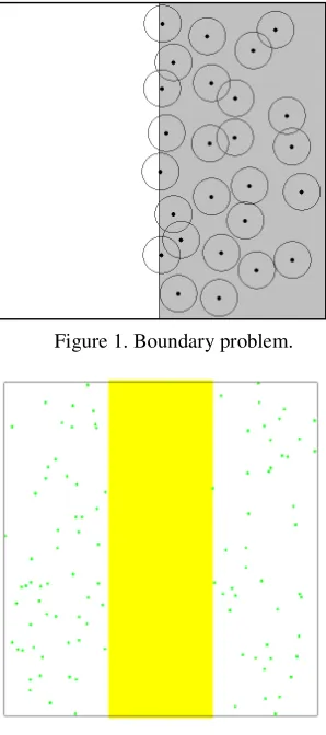
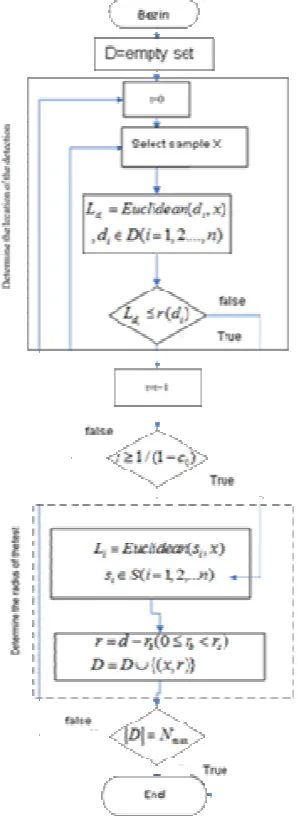
paper, the former is called "radical (aggressive)", the latter is "conservative". It is clear that each of the points can be used as a proof of the self region near the region. On the other hand, from the perspective of fairness, it is assumed that the self points can be obtained from any part of the whole body. Therefore, no matter which matching rules are used, the points that are close to the boundary of the self and non self region cannot be ignored. That is, how to generalizing the self and non self boundary of the autologous sample is a difficult problem. Therefore, it is difficult to make a reasonable explanation of these elements. Figure 1 shows the boundary problem. The shaded part said actual self region, the white area said non self region and dots indicate self data, circle is autologous generalization. As can be seen from Figure 1, the self sample points close to the boundary inevitably extend the range of the actual self region algorithm. If the threshold is too small, the space between the samples will not be expressed, in other words, more samples will be needed to train the system. If the threshold is too large, the error of the self region is too large to be accepted. In particular, when the nonself region is in two regions of autologous thin strips, as shown in Figure 2, there may simply cannot be said (yellow bar indicates the non self region). In this case, the boundary problem is more serious. Therefore, it is necessary to design a new algorithm to solve the boundary problem.
Figure 1. Boundary problem.
Figure 2. Banded non self.
3. BASIC STEPS OF ALGORITHM AND ANALYSIS
3.1 Basic steps of algorithm
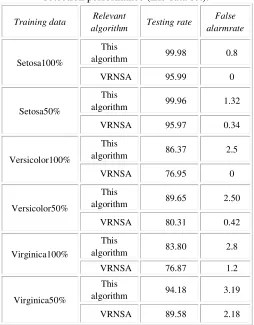
In this paper, the design of the detector generation algorithm, the basic steps are outlined as follows. Where S represents a collection of self samples;
max
N represents the maximum number of preset detectors; rs represents the self radius; a is the desired coverage. D Representing the generated detector set, d ii( =1, 2,... )n is a detector in the detector set; t is a random sample points covered by detector.
Step 1: generate candidate detectorx (using a combination of [9] and random generation from the gene pool);
Step 2: calculate the Euclidean distance between the x and the detector d i(i =1, 2,... )n in the
detector set ( , )
i
d i
L =Euclidean d x ;
Step 3: if the distance
i
d
L is less than the radius
( )i
r d of the detector di, the point x has been covered by the detector, then the counter t= +t 1; otherwise the turn step 5;
Step 4: ift≥1 / (1−a) , then the coverage is sufficient, the end of the algorithm; otherwise, turn step 1;
Step 5: computing point x and self point
i
s from Autologous sample set S ,it’s Euclidean distance is Li=Euclidean s x( , )i , x radius r is determined by the recent self elements, remembering distance from x recent self point distance d detector ( , )x r which r=d−rb(0≤rb <rs); rb said as the threshold boundary control parameters, is used to control the detector "aggressive";
Step 6: add the ( , )x r as a new detector to the detector setD;
Step 7: if the detector set D to the maximum
number of detectors Nmax, then the end; otherwise; turn step 1
Figure 3. Basic flow chart of algorithm.
3.2 Algorithm characteristics and advantages analysis
(1) The biggest difference of this algorithm lies in: This paper sets a boundary threshold rb to measure the aggressiveness of boundary detector in the self region boundary. We can use the rb size of the different, to control the performance of the algorithm.
(2) Compared with the fixed length detector [3], the radius of each detector in this algorithm is variable. Due to the variable radius, the algorithm has better coverage ability to detect "black hole".
(3) And VRNSA compared [4], the algorithm in selecting the candidate detectors are proposed by combination of randomly generated and the gene pool, both to ensure the diversity of the detectors, and improve the production efficiency of the detectors, and detection rate can be increased.
(4) The detector generates an integrated coverage estimation method, which is used as the termination condition of the algorithm, rather than simply
depends on the maximum number of preset detectors. Therefore, this algorithm provides the following two ways: the first case is: when the estimated coverage of the algorithm, which is the end of the algorithm, this algorithm is unique, you can avoid the production of redundant detectors. The second case is: the number of detectors to reach the preset value. Even in this case, because the detector is longer, the algorithm still has the ability to better cover the black hole. The correctness of the point estimate (step 4) is shown as follows:
1) Generating random points as candidate detectors;
2) If it is a non self point and is not covered, on top of it produced a new detector; if it is covered by the self point is not as the candidate detector, but attempt was recorded in a counter t to estimate coverage;
3) If sampling m points in the non self space, there is only one point that has not been covered, by point estimation, the non covered area is: 1/m, the coverage rate is estimated as: a= −1 1 /m;
4) Therefore, when a random attempt is made to t times without finding an uncovered point (point all covered), the actual coverage rate has been estimated to bea. Therefore, t does not need to default, it is determined by the target coverage rate:
1
1
t
a
=
−
4. EXPERIMENT AND RESULT ANALYSIS
In order to verify the performance of the algorithm, experiments on both synthetic data and real data are carried out to verify the performance of [10-11], and compared with the related algorithms.
4.1 Results on synthetic data
is Nmax=1000, rs=0.1, a=99%, the threshold of 0.01-0.1. The result of the experiment is to use the same parameter to run 100 times. Detection performance using the detection rate (rate detection) and false alarm rate (alarm rate false) to measure. Contrast algorithm for the classic [4] algorithm VRNSA.
The experimental results are shown in figure 4.
Figure 4. Experimental results.
[image:4.612.60.296.152.301.2]In the figure, the horizontal coordinates represent the boundary threshold, and the longitudinal coordinates respectively represent the detection rate and false alarm rate. As can be seen from the figure, with the increase of the boundary threshold, the detection rate of the algorithm is reduced, while the false alarm rate is also reduced. Mainly due to: with the change of the boundary threshold, the algorithm detects the small radius of the detector which is close to the edge of the non self space. From the figure can be seen, the detection rate of the proposed algorithm is much higher than the VRNSA [4] algorithm, the false alarm rate is slightly increased. The main reason is that: in the VRNSA algorithm, a large part of the non self will be used as a body, therefore, reduce the detection rate. Considering synthetically, the algorithm has certain advantages. At the same time, the boundary threshold is adjustable, which can be used to balance the detection rate and false alarm rate.
4.2 Experimental results on real data
In order to verify the performance of the algorithm, the well-known Iris Fisher's data set is used to compare with other related algorithms [11].The data set has 3 classes, each class of 50 samples, each sample is a 4 dimensional feature vector. Are the mountain (Iris setosa), iris iris versicolor (Iris versicolor) and Virginia (Iris virginica). When the experiment, a kind of data is used as the normal data, the other two kinds of abnormal data. Normal data is used to train the system. Among them, 50% of the Setosa said setosa is considered normal data, the other two types (versicolor and virgnica) was as
abnormal data, 50% setosa data is used as training data, all three types of data (including has been used as training data) as the test data and other (Setosa 25 percent) said that the meaning is similar. The results of the experiment are the results of the 100 repeated experiments for each method and the parameter settings. And set the same experimental parameters with other algorithms in order to compare. The results of the experiment are shown in table 1.
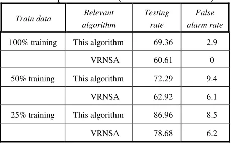
Table 1. Comparison of correlation algorithm detection performance (Iris data set).
Training data Relevant
algorithm Testing rate
False alarmrate
Setosa100%
This
algorithm 99.98 0.8
VRNSA 95.99 0
Setosa50%
This
algorithm 99.96 1.32
VRNSA 95.97 0.34
Versicolor100%
This
algorithm 86.37 2.5
VRNSA 76.95 0
Versicolor50%
This
algorithm 89.65 2.50
VRNSA 80.31 0.42
Virginica100%
This
algorithm 83.80 2.8
VRNSA 76.87 1.2
Virginica50%
This
algorithm 94.18 3.19
VRNSA 89.58 2.18
As can be seen from the table, the algorithm compared with [3] VRNSA, the detection rate has been greatly improved, false alarm rate increased slightly, can effectively improve the detection efficiency.
[image:4.612.309.563.176.501.2]important parameter for the balanced detection rate and the false alarm rate.
Table 2. Comparison of correlation algorithm detection performance (Biomedical data set).
Train data Relevant algorithm
Testing rate
False alarm rate
100% training This algorithm 69.36 2.9
VRNSA 60.61 0
50% training This algorithm 72.29 9.4
VRNSA 62.92 6.1
25% training This algorithm 86.96 8.5
VRNSA 78.68 6.2
5. CONCLUSIONS
In this paper, we propose a new algorithm of edge detection based on the shortcomings of the existing detector algorithm in dealing with the boundary element, and the advantage of the algorithm is verified by the synthetic data and the actual data. In practical use, the specific parameter values depend on the specific application problems. The next research work is: how to automatically determine these parameters, such as the radius of rs, the
boundary threshold rb, etc.
REFERENCES
[1]Mo Hongwei, Zuo Xingquan. Artificial immune system [M]. Beijing: Science Press, 2009
[2]M. Bereta and T. Burczy humorous nski. comparing binary and real-valued coding in hybrid immune algorithm for feature selection and classification of ecgsignals. Eng. appl. Artif. Intell., of 20 (5): 571 - 585, August 2007.
[3]Gonzalez, F., D.Dasgupta, F. Nino L., Randomized Rea-Valued Negative Selection Algorithm A, ICARIS-03. 2005 [4]ZHOU JI DASGUPTA D. Real-valued negative selection
algorithm with variable-sized detectors[C]Proceedings of GECCO LNCS 3102 Berlin:. Springer, 2007: 287-298. [5]Z. Ji and D. Dasgupta. applicability issues of the
real-valued negative selection algorithms. in genetic and evolutionary computation Conference (GECCO 2006), pages 111 - 118, Seattle, Washington, 8-12 July 2007. [6]Gonzalez, F., Dasgupta D., Detection Using Real-Valued
Negative Selection Genetic, Programming and Evolvable Machine Anomaly, 4 383-403, 2006
[7]Stibor T., Timmis J., C. Eckert. A comparative study of negative real-valued and selection to statistical anomaly detection techniques.In ICARIS pages, 262 - 275, 2005. [8]Yang Dongyong, Chen Jinyin. Based on multi-population
genetic algorithm of detector generating algorithm [J]. Automation of Chemistry, 2009, 31 (4):1407-1410. [9]Zhu Sifeng, Liu Fang, Chai Zhengyi. Based on the Journal
of detector coverage evaluation of negative selection algorithm [J]. Huazhong University of Science and Technology (Natural Science Edition), 2009, 31 (12):1407-1410.
[10] Columbia University.2DSyntheticData [EB/OL]. [2010-3-12]. http:// www.zhouji.net/prof/2DSyntheticData.zip. Datasets Archive