Rheological Measurements in Liquid Solid Flows

(1)

Thesis by

Erin Koos

In Partial Fulfillment of the Requirements for the Degree of

Doctor of Philosophy

California Institute of Technology Pasadena, California

2009

(2)

(3)

Acknowledgements

When I look back at my time here at Caltech, I know it would not have been possible without the help I received along the way.

First, I would like to thank Professor Melany Hunt, my advisor, for her guidance and support. From my first day in her lab to these very last days, her door has always been open to answer questions, give encouragement, and offer an understanding ear. Melany gave me the support I needed when nothing seemed to work allowing me to eventually succeed. I would also like to express the gratitude I have for the help and motivation I received from Professor Christopher Brennen. On everything from the practical to the theoretical, he would always have time to help with my questions – each meeting ending with the ever present “press on."

I also extend my thanks to Prof. John F. Brady, Prof. Joseph E. Shepherd, and Prof. Roberto Zenit for serving on my committee and reviewing my dissertation. I appreciate their time and comments. Each red mark was a chance to make the finished product that much better.

I also owe a debt of gratitude to Dr. Jim Cory. Jim designed and had constructed the apparatus used for these experiments. It has undergone a few small redesigns since, but the bulk of the experiment is still his work. I would also like to express my thanks to Esperanza Linares for helping me with some of my measurements; I wish you luck in your future experiments. Angel Ruiz-Angulo served as my mentor and made me feel welcome not to mention supplying me with many samples of apple cake as he perfected his recipe. To the other members of the Granular Flows Group, both past and present, thank you.

(4)

needed to redesign components, I’d usually end up in John’s office asking him if the idea was feasible (or advisable). I would also like to thank Candace Rypisi and Felicia Hunt as directors of the Women’s Center for providing a welcome home, weekly lunches and an always sympathetic ear. Many thanks are also extended to the many other members of the Caltech community without whom, my experiences as both a student and researcher would have been hindered.

Without my friends here at Caltech and elsewhere, my life would be much diminished. Adam Mills was always available when I needed a soft shoulder or to escape for a week-end. Maybe one day, I’ll be able to answer my own "should I" questions. I will always remember tramping through the woods with Anna Folinsky. In summer and winter, you put up with my slow pace (and occasional blisters). I would certainly have been less active and seen much less of California were it not for you. Dr. Jennifer Stockdill, creative ge-nius, my kitchen is always open for you; invite yourself over any time. Dr. Deepak Kumar, thank you for all of your help and the many relaxing meals I was able to share with you. You need to take me up flying when you finish your pilot’s license. Jenny Roizen, you are one of the kindest people I know: from my very first day on campus, you have been there whenever I needed a hug or to go out and have fun.

(5)

Abstract

This thesis presents experimental measurements of the shear stresses of a fluid-particulate flow at high Reynolds numbers as a function of the volume fraction of solids. From the shear stress measurements an effective viscosity, where the fluid-particulate flow is treated as a single fluid, is determined. This viscosity varies from the fluid viscosity when no solids are present to several orders of magnitude greater than fluid viscosity when the par-ticles near their maximum packing state. It is the primary goal of this thesis to determine how the effective viscosity varies with the volume fraction of solids.

A variety of particle sizes, shapes, and densities were obtained through the use of polystyrene, nylon, polyester, styrene acrylonitrile, and glass particles, used in configu-rations where the fluid density was matched and where the particles were non-neutrally buoyant. The particle sizes and shapes ranged from 3 mm round glass beads to 6.4 mm nylon to polystyrene elliptical cylinders. To properly characterize the effect of volume tion on the effective viscosity, the random loose- and random close-packed volume frac-tions were experimentally determined using a counter-top container that mimicked the

in situ(concentric cylinder Couette flow rheometer) conditions. These volume fractions

depend on the shape of the particles and their size relative to the container.

The effective viscosity for neutrally buoyant particles increases exponentially with vol-ume fraction at fractions less than the random packing. Between the random loose-and rloose-andom close-packed states, the effective viscosity increases more rapidly with vol-ume fraction and asymptotes to very large values at the close-packed volvol-ume fraction. The effective viscosity does not depend on the size or shape of particles beyond the influence these parameters have on the random packing volume fractions.

(6)

the shear rate of the Couette flow and decreases with the Archimedes number in a way that when plotted against the Reynolds number over the Archimedes number, these curves col-lapse onto one master curve. When the local volume fraction is used, the effective viscosity for non-neutrally buoyant particles shows the same dependence on volume fraction as the neutrally buoyant cases.

(7)

List of Figures

1.1 Critical Reynolds number for the onset of Couette-Taylor flow . . . 5

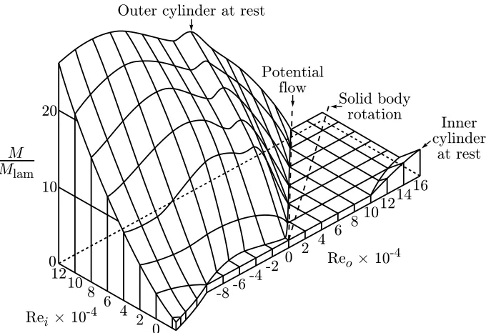
1.2 Increase in torque for inner and outer rotating Couette flows . . . 5

1.3 Critical Reynolds number for the onset of turbulence in pipe flow with particles 7 1.4 Phase diagram for non-Brownian fluid-particulate flows . . . 8

1.5 Experimental apparatus used in Bagnold (1954, 1956) . . . 12

1.6 Reynolds number-volume fraction phase diagram of previous experiments . 15 1.7 Experimental apparatus used in Savage and McKeown (1983) . . . 15

1.8 Experimental apparatus used in Acrivos et al. (1994); Hanes and Inman (1985); Prasad and Kytömaa (1995) . . . 17

2.1 Dilatancy of particles . . . 22

2.2 Hexagonally close-packed spheres . . . 24

2.3 Images of random packing in a confined container . . . 27

2.4 Oscillation of the volume fraction near a wall . . . 28

2.5 Influence of finite containers on the volume fraction of round particles . . . . 29

2.6 Approximations for close- and close-packing for nearly spherical particles . . 31

3.1 Coaxial rotating cylinder, Couette flow device . . . 38

3.2 Typical response curve for the MTI KD-300 fotonic sensors used with a MTI 0623H optical probe . . . 41

3.3 Schematic of the optical probe configuration to measure particle counts and velocities . . . 42

3.4 Bode magnitude plot for the combined lowpass and bandstop filter . . . 43

(12)

3.6 Filtered and normalized voltage signal from two probes located in the lower

observation port . . . 45

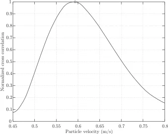
3.7 Converted voltage signal used for the cross-correlation of the full voltage sig-nals for two adjacent optical probes . . . 46

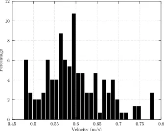
3.8 Normalized cross-correlation amplitude showing the likely particle velocities 47 3.9 Histogram of particle velocities found using thecorrel.mfunction . . . 48

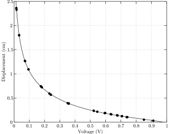
3.10 Post peak displacement as a function of normalized voltage for the MTI opti-cal displacement sensors . . . 49

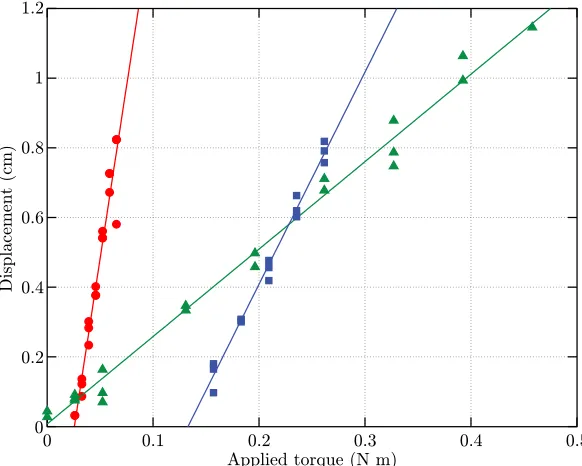
3.11 Spring stiffness for three different springs . . . 50

3.12 Pure fluid calibration . . . 52

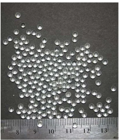
3.13 The glass spheres used in the rheological experiments . . . 54

3.14 Histogram of glass particle sizes . . . 55

3.15 The nylon spheres used in the rheological experiments . . . 55

3.16 Histogram of nylon particle sizes . . . 56

3.17 The polyester scalene ellipsoids used in the rheological experiments . . . 57

3.18 Histogram of polyester particle sizes . . . 58

3.19 The polystyrene elliptical cylinders used in the rheological experiments . . . 59

3.20 Histogram of polystyrene particle sizes . . . 59

3.21 The SAN scalene ellipsoids used in the rheological experiments . . . 61

3.22 Histogram of SAN particle sizes . . . 61

4.1 Shear stress measurements for suspensions of polystyrene particles in aque-ous glycerine . . . 66

4.2 Ratio of measured-to-pure fluid torques for suspensions of polystyrene parti-cles in aqueous glycerine . . . 67

4.3 Effective viscosity ratio for neutrally buoyant polystyrene particles in aque-ous glycerine solutions . . . 68

4.4 Deviation from the mean effective viscosity ratio . . . 69

4.5 Shear stress measurements for suspensions of nylon particles in aqueous glyc-erine . . . 70

(13)

4.7 Effective viscosity ratio for neutrally buoyant nylon particles in aqueous glyc-erine solutions . . . 72 4.8 Shear stress measurements for neutrally buoyant SAN particles in aqueous

glycerine . . . 73 4.9 Ratio of measured-to-pure fluid torques for suspensions of SAN particles in

aqueous glycerine . . . 74 4.10 Effective viscosity ratio for neutrally buoyant SAN particles in aqueous

glyc-erine solutions . . . 75 4.11 Effective viscosity for neutrally buoyant particles in aqueous glycerine . . . . 76 4.12 Effective viscosity for neutrally buoyant particles in aqueous glycerine . . . . 77

5.1 Graph of the particle velocity obtained from optical probes mounted on the stationary inner cylinder . . . 82 5.2 Graph of the normalized particle velocity obtained from optical probes . . . . 83 5.3 Histogram of velocity fluctuations . . . 84 5.4 Standard deviation in particle velocity normalized by the mean value . . . . 85 5.5 Graph of the particle counts obtained from optical probes mounted on the

stationary inner cylinder . . . 86 5.6 Volume fraction across the floating cylinder for various aqueous glycerine

solutions . . . 87 5.7 Volume fraction across the floating cylinder as a function of the Reynolds

number divided by the Archimedes number . . . 89 5.8 Shear stress measurements of polystyrene particles in varying concentrations

of aqueous glycerine . . . 90 5.9 Ratio of measured-to-pure fluid torques of polystyrene particles in varying

concentrations of aqueous glycerine . . . 92 5.10 Effective viscosity ratio as a function of the density of the interstitial fluid

normalized by the particle density . . . 93 5.11 Effective viscosity ratio for both neutrally buoyant and non-neutrally

(14)

5.13 Coefficient of friction versus the gap Reynolds number divided by the Archimedes

number . . . 96

5.14 Shear stress measurements for non-neutrally buoyant glass particles in aque-ous glycerine . . . 97

5.15 Ratio of measured-to-pure fluid torque for non-neutrally buoyant glass par-ticles in aqueous glycerine . . . 98

5.16 Shear stress measurements for non-neutrally buoyant polyester particles in aqueous glycerine . . . 99

5.17 Ratio of measured-to-pure fluid torques for non-neutrally buoyant polyester particles in aqueous glycerine . . . 100

5.18 Effective viscosity ratio for neutrally buoyant polyester particles in aqueous glycerine solutions . . . 101

5.19 Effective viscosity for all particles . . . 102

5.20 Effective viscosity for all particles compared with other experimental data . . 103

5.21 Theoretical curve fits for dilute particle concentrations . . . 104

5.22 Curve fits using experimentally determined fitting parameters . . . 106

6.1 Types of slip occurring near a smooth wall . . . 108

6.2 Typical depletion layer thicknesses . . . 109

6.3 Ratio of the apparent viscosity to the actual bulk viscosity for several deple-tion layer thicknesses . . . 113

6.4 Photograph of typical surface roughness . . . 115

6.5 Shear stress measurements for suspensions of polystyrene particles in aque-ous glycerine with rough cylinder walls . . . 117

6.6 Ratio of measured torque to pure fluid torques for suspensions of polystyrene particles in aqueous glycerine with rough cylinder walls . . . 118

6.7 Effective viscosity ratio for neutrally buoyant polystyrene particles in aque-ous glycerine solutions with rough cylinder walls . . . 120

6.8 Depletion layer thicknesses calculated from apparent and actual viscosity measurements . . . 121

(15)

6.10 Depletion layer thickness calculated from the velocity measurements shown as a function of the Reynolds number . . . 123 6.11 Depletion layer thickness calculated from velocity measurements . . . 124 6.12 Particle velocity near the stationary wall for smooth and rough walls . . . 125 6.13 Smooth wall data corrected for the presence of particle depletion layers . . . 127

(16)

(17)

List of Tables

1.1 Previous experiments on non-Brownian shear flows . . . 14

2.1 Random close-packing volume fraction . . . 25

2.2 Random loose-packing volume fraction . . . 26

2.3 Random packing volume fractions for current particles . . . 32

2.4 Previous experiments of non-Brownian shear flows . . . 33

3.1 Dimensions and properties of the rotating cylinder rheometer . . . 39

3.2 Properties for experiments . . . 53

(18)

(19)

Nomenclature

Greek Characters

β Volume quality

˙

γ Shear rate of the interstitial fluid

δ Perturbation in the diameter of a nearly spherical particle

µ Viscosity of the interstitial fluid

µ0 Effective viscosity for the fluid-solid mixture

ρf Density of the interstitial fluid

ρp Particle density

τ Shear stress for the fluid-solid mixture, usually as measured on the inner, floating cylinder

φ Volume fraction of solids

φc Volume fraction of solids at random close-packing

φl Volume fraction of solids at random loose-packing

Ω Angular velocity of outer rotating cylinder

Latin Characters

Ap Surface area of an individual particle

Ar Archimedes number,Ar =gd3ρf |ρp−ρf |/µ2

(20)

Ba Bagnold number,Ba =λ12ρ_pd2γ/µ˙

Cf Coefficient of friction,Cf = 4τ /(ρfγb˙ 2)

Ci Displacement fit coefficients

D Spring displacement

d Particle diameter

dlarge Largest measured particle diameter

dsmall Smallest measured particle diameter

E Voltage measured from the optical displacement probes

g Gravitational acceleration,g= 9.81m/s2

H Height of the floating cylinder,H= 11.22cm (4.42 in)

h Height of the annulus,h= 36.98cm (14.56 in)

k Boltzmann constant

L Average particle separation

l Particle length for cylindrical particles

M Torque generally or as measured on the inner, floating cylinder

Mf luid Torque calculated using the fluid viscosity

n Number of particles per unit time

p Pressure for the fluid-solid mixture

Pe Péclet number,Pe = 3πµd3γ/˙ 4kT

r Radial coordinate

Re Reynolds number,Re =ρfγd˙ 2/µ

(21)

Reb Gap Reynolds number,Reb=ρfγb˙ 2/µ

ri Radius of the inner drum,ri = 15.89cm (6.26 in)

ro Radius of the outer drum,ro = 19.05cm (7.50 in)

St Stokes number,St =ρpγd˙ 2/(9µ)

T Effective stress tensor for the fluid-solid mixture

T Temperature

u Particle velocity

V Velocity of the outer, rotating cylinder

Vp Volume of an individual particle

(22)

Chapter 1

Introduction

Fluid-solid flows are observed in a variety of fields ranging from mining operations to the erosion of the Martian landscape. Particulate flows help polish and cut metals in manufac-turing practices, but are also associated with the rapid deterioration of industrial compo-nents. The mechanics of particulate flows cause dune formation and determine the dam-age caused by a landslide. These are just a few examples of the vast range of fluid-solid material flows of interest to engineers and scientists.

(23)

1.1

Flow regimes

In general, fluid-solid flows are associated with the movement of particles through an interstitial fluid where the viscous effects of the fluid, the inertia of the fluid and particles, and the collisions between particles all contribute to the mechanics. In addition to these mechanisms, additional forces associated with many particles in the fluid (e.g. lift, drag, added mass) may also significantly change the mechanics of the flow.

To investigate the nature of these fluid particulate flows, particles with diameterdand densityρpare placed in a Couette flow device consisting of two concentric cylinders (with

shear rateγ˙ and gap widthb) filled with a Newtonian fluid with viscosityµand density

ρf. This fluid-solid flow can be characterized by an effective stress tensorTcomposed of

shear stressτ and pressurep. To simplify the form of the stress tensor, it is hypothesized that the fluid-solid mixture is also Newtonian, thus

τ =µ0γ,˙ (1.1)

where µ0 is the effective viscosity of the fluid-solid mixture. This effective viscosity de-pends on the properties of the fluid, the properties of the solid, the fluid shear rate, the gap width, the volume fraction of solidsφ, and thermal energykT:

µ0 =f(µ, ρf, ρp, d, g,γ, b, φ, kT˙ ). (1.2)

Reducing this dependance to non-dimensional parameters,

µ0 µ =f

φ,Re,Pe,Ar,ρp ρf

,d b

, (1.3)

where the Reynolds number, the ratio of fluid inertial force to the fluid viscous force, is defined by

Re =ρfγd˙ 2

µ , (1.4)

for a Couette flow. The Reynolds number is an indicator for the onset of turbulence and the existence of secondary flows. The Peclét number, the ratio of particle advection to thermal diffusion, is defined by

Pe = 3πµd

3_γ_˙

(24)

The Archimedes number

Ar = gd

3_ρ

f|ρp−ρf|

µ2 , (1.6)

describes the ratio of gravitational forces to viscous forces. The remaining non-dimensional parameters areρp/ρf, the ratio of the particle-to-fluid density, andd/b, the ratio of the

par-ticle diameter to the gap width.

The equation for the effective viscosity, equation (1.3), can be simplified by employing a few key assumptions. In the following subsections, several of these assumptions are discussed in more detail.

1.1.1 Continuum assumptions

Inherent in the examination of bulk fluid properties is the assumption that the flow is a continuum: enough particle-particle and particle-wall collisions occur during a measure-ment so that their effect is averaged. Furthermore, it is argued that the results are not affected by the presence of the cylinder walls. For the continuum assumption to hold, lim-its must be placed on the volume fraction of particles φand on the ratio of gap width to particle diameter,b/d. The volume fraction must be large enough so that, over the time of the experiments, a sufficient number of particle collisions occur. In the present experiment, the volume fraction of solids was larger than 0.05, for which the continuum assumption should hold.

Appropriate limits on the ratio of gap width to particle diameter are more difficult to determine. The slip of particles against the cylinder walls causes a lower effective shear rate within the bulk of the fluid-particulate mixture. A general rule for experiments with suspensions of particles in a fluid is that the gap width must be at least 10 times the particle diameter (Barnes 1995). In the current experiments, the ratiob/dis often close to this limit of 10 (e.g. 9.5 for the polystyrene particles). The nature of slip on the outer walls and its influence on shear stress measurements are discussed in chapter 6.

(25)

to the gap between the concentric cylinders. (The height and width of the box are much greater than the gap and should not change the volume fraction). See section 2.2 for a detailed discussion of this behavior.

1.1.2 Secondary flows

The radial inertia due to a rotating flow can induce a radial velocity in the fluids and particles. At low Reynolds numbers, the viscosity can suppress this radial velocity, but as the Reynolds number increases, Taylor vortices develop. As with single component flows, secondary flows and turbulence can develop in fluid-particulate flows. In a concentric cylinder Couette flow where the outer rotates and the inner cylinder is held stationary, secondary flows are present in the form of Taylor vortices and the boundary layer flows near the end caps. These secondary flows increase the shear stress on the cylinder walls and, without correction, can yield a higher effective viscosity than without these effects.

The growth of Taylor vortices depends on the geometry of the annular gap as well as the rotational velocity of both the inner and outer cylinders. Even in the case of a granular flow, where the fluid effects are negligible, Taylor-like vortices develop at a slightly lower Reynolds number than in the fluid case (Conway et al. 2004). The vortices develop at a much lower Reynolds number for a Couette flow with the inner cylinder rotates than for a flow where the inner cylinder is fixed and the outer cylinder rotates. The data obtained by Taylor (1936a,b), shown in Figure 1.1, shows this trend very clearly. As the gap widthbis increased relative to the inner cylinder radiusri, the critical Reynolds number for the

on-set of Taylor-Couette vortices decreases for inner rotating Couette flows and increases for outer rotating Couette flows. The presence of Taylor-Couette vortices can greatly increase the observed torque in a nonlinear manner, as shown in Figure 1.2. Even small errors in the Reynolds number can lead to large changes in the pure fluid torque. The effective viscos-ity of the fluid-particulate mixture is calculated relative to pure fluid viscosviscos-ity through the normalization of the measured to pure fluid torque. Through this normalization, small un-certainties in the Reynolds number can create significant errors in the normalized effective viscosity measurement. Due to this possible error, care is taken to avoid Taylor-Couette flows in the present experiment.

(26)

an-103

Critical Reynolds number

105

104

102

b/r_i

10¹3 ₁₀¹2 ₁₀¹1 ₁₀0

Inner rotating cylinder Outer rotating

[image:26.612.154.490.82.351.2]

cylinder

Figure 1.1. Critical Reynolds number for the onset of Couette-Taylor flow for both inner and outer rotating cylinders as a function of the ratio of gap width to inner radius. (Taylor 1936a).

Re_i£ 10-4

0 2 4 6 8 12

10

Re_o£ 10-4 0 2

4 6 8

12 10

-2 -4 -6 -8

1416

0 10 20

M_lam M

Inner cylinder

at rest Potential

flow

Solid body rotation Outer cylinder at rest

Figure 1.2. Increase in torque for inner and outer rotating Couette flows forb/ri = 0.176

[image:26.612.155.495.432.665.2]

(27)

nulus. The inertial opposition to the centripetal acceleration is balanced by a pressure gradient in the center of the flow. An axial gradient exists near the end caps due to the non-slip condition, which disrupts the pressure gradient. This resultant force near the end caps drives a radial flow close to the boundary (Czarny et al. 2003). When the end caps are fixed, these boundary layers are termed Bödewadt flows, or termed Ekman boundary layers when the end caps and flow are rotating at different angular velocities (Lingwood 1997). As the rate of rotation increases, the boundary layers decrease in size but increase in strength, inducing counterrotating recirculation cells. These cells grow with the increasing Reynolds number until they eventually meet at the midplane. The boundary layer and its accompanying recirculation cell has an increasing influence on the torque measurements.

The influence of particles on the development or strength of secondary flows is another source of uncertainty. Experimental results summarized in Gore and Crowe (1991) show that turbulence is strengthened by small particles and attenuated by large particles. This attenuation is due in part to particle-fluid and particle-particle-fluid coupling, the magni-tude of which is influenced by the volume fraction of particles (Elghobashi 1994). These two effects are summarized in the data from Matas et al. (2003), which looks at the critical Reynolds number for the onset of turbulence in horizontal pipe flow (Figure 1.3). A sim-ilar influence of the volume fraction is expected for the initiation of Taylor vortices or on boundary layer flows. The effect of particles on secondary flows is difficult to estimate, making comparisons between single phase experiments at the same Reynolds number problematic. The added complexity caused by these secondary flows should be avoided.

1.1.3 Diffusion and Brownian motion

The diffusion of particles in a fluid is governed by advection, particle interactions, and thermal diffusion. Advection – diffusion caused by a fluid velocity gradient – depends on how quickly the Couette flow is being sheared; diffusion due to particle interactions is a function of the volume fraction of particles in the fluid; thermal diffusion is a function of the fluid temperature. Diffusion always occurs, but the dominant type of diffusion may change.

(28)

tem-0 0.05 0.1 0.15 0.2 0.25 0.3 0.35 0.4 103

104

Critical Reynolds number

Á d/D = 0.0029 § 0.0003

d/D = 0.015 § 0.002 d/D = 0.021 § 0.002 d/D = 0.037 § 0.004 d/D = 0.056 § 0.006 d/D = 0.063 § 0.008 d/D = 0.10 § 0.01

Figure 1.3. Critical Reynolds number for the onset of turbulence in pipe flow as a function of the volume fraction of solidsφand the ratio of particle diameter to pipe diameterd/D. Turbulence is delayed for smaller particles and high volume fractions (Matas et al. 2003).

perature increases and as the particle diameter decreases, the Brownian motion of particles becomes more pronounced. At room temperature, particles with diameters smaller than 100 µm show clear Brownian motion while particles with diameters greater than 1 mm do not. The ratio of advection to thermal diffusion is termed the Peclét number (equa-tion (1.5)). For processes with Peclét numbers that are very large (Pe → ∞), the system is not subjected to Brownian diffusion. Generally, systems withPe & 103 are considered non-Brownian (Stickel and Powell 2005). In all of the experiments considered in this the-sis, the particle sizes are large enough and the fluid is moving sufficiently quickly that the flows are considered non-Brownian. Then, the effective viscosity depends only on the other non-dimensional parameters, µ_µ0 =fφ,Re,Ar,ρp

ρf,

d b

.

(29)

non-collisional flows is currently unclear and one of the goals of this thesis is to determine this transition. A further discussion of the transition toward the continuous contact regime can be found in chapter 2.

1.1.4 Phase diagrams

Since Bagnold (1954, 1956) first explored fluid particulate flow in his concentric Couette experiment, other researchers have looked at different aspects of these flows. Generally, these experiments can be placed in several categories. The most basic differentiation of these categories is shown in Figure 1.4(a), which shows the phase diagram of volume frac-tion and of Archimedes number relative to the Reynolds number. The continuous contact

Re

Á

Ácrit

Recrit 0

Continuous contact

Secondary flows Laminar

(a)

Sliding bed

Heterogeneous suspension

Saltation

Homogeneous suspension

Re Recrit

Secondary flows

Ar

0

(b)

Figure 1.4. Phase diagram for non-Brownian fluid-particulate flows. As a function of the Reynolds number, the influence of (a) volume fraction and (b) Archimedes number are shown on the behavior of the flow. These figures are based on the work of Coussot and Ancey (1999) and King (2001).

regime comprises flows where the particles are always in contact and collisional diffusion dominates over advection. Above a critical Reynolds number, secondary flows are present. These secondary flows greatly complicate the flow behavior and can contribute to a higher observed torque. Since the particles can alter these secondary flows, comparisons between single phase and particle laden cases are complicated. This regime is avoided in this the-sis. The third region comprises laminar flow without secondary flows where advection dominates.

(30)

the behavior of the fluid-particulate flow. As the density difference between the particles and fluid is increased, the Archimedes number increases and a higher Reynolds number is required to fluidize the bed (Bi and Fan 1992; King 2001). Particle mixtures undergoing saltation or in a heterogeneous suspension show variations in the local volume fraction in the axial direction. A variation in the effective viscosity, due to this volume fraction gradient, can complicate the dynamics of the flow. In the present experiments, when the particle density and fluid density were not matched (chapter 5), the volume fraction was measured locally. Thus, if the particles are not in a homogeneous mixture, the effective viscosity can be correlated directly with the local volume fraction.

In addition to the phase diagram for variations in the volume fraction and Archimedes number, variations in Peclét number can also be considered. For low Peclét numbers, the flow is Brownian and thermal diffusion dominates. As the Peclét numbers for the experi-ments discussed in the following chapters are all much larger than unity, any rheological effects in this region are small and are neglected.

1.1.5 Particle interactions

Individual interactions between two colliding particles can vary dramatically based on the relative inertia of the particles and the elasticity of the particles. Particle collisional behavior is characterized by the Stokes number, which describes the ratio of particle inertia to fluid viscous forces,

St = ρpureld

9µ (1.7)

(Joseph and Hunt 2004; Joseph et al. 2001). For shear flows, the relative velocity between two adjacent particles is approximately equal to the shear rate times the distance between the two particle centers. This separation between two adjacent particles is close to particle diameter. The Stokes number for this flow is related to the Reynolds number by

St = ρpγd˙ 2

9µ (1.8)

= 1

9 ρp ρf

Re. (1.9)

(31)

num-ber less than about 10 (Joseph and Hunt 2004; Joseph et al. 2001). For collisions between two particles, a Stokes number based on the relative velocities between the two particles is chosen. As shown in Yang (2006); Yang and Hunt (2006), for small Stokes numbers (St .2), the slow particle began to move as the fast particle approached and there was no clear collision. For slightly larger Stokes numbers (St≈3−9), there was a clear collision, but no rebound: the two particles travel as a single composite particle following the colli-sion. At larger Stokes numbers, there was a clear rebound between the two particles. For oblique collisions, the normal collisional interaction proceeds just as described above, but the ratio of incident to rebound angle vary with Stokes number.

The collision of a particle with either a wall or a second particle is associated with en-ergy dissipation due to the inelasticity of the contacts. This enen-ergy dissipation is described by the coefficient of restitution: the ratio of the rebound velocityvrto the incident velocity vi,

e=−vr

vi

(1.10)

for a collision against a stationary wall. For a collision between a second particle, the relative velocities must be used. The coefficient of restitution, which must be a function of Stokes number and the properties of the two materials as is shown in Ruiz-Angulo (2008). For steel particles against a Zerodur wall, where both the wall and particles have high Young’s moduli, the coefficient of restitution is well described by the empirical fit

e= 1− 8.65

St0.75 (1.11)

as shown in Joseph (2003) and represents the elastic limit. For collisions involving greater plastic deformation, the coefficient of restitution will decrease. The elastic velocity is de-fined as

uel=

π2 2E∗2p

10ρp

(1.65Y)5/2 (1.12)

where Y is the yield strength and E∗ is the reduced modulus, defined as E∗ = [(1−

ν₁2)/E1+(1−ν22/E2]−1, which depends on the Young’s modulus for each materialEias well

as Poisson’s ratioνi. For particle-particle collisions within the fluid, the two materials are

(32)

section 3.3. For the materials used and the range of Stokes numbers tested, a reduction of less than 10% in the coefficient of restitution will occur.

1.2

Previous experiments

Bagnold (1954) first experimented with the rheology of fluid-particulate flows and pro-posed a non-dimensional number to govern variations between a rapidly sheared, high volume fraction region and a slow, low volume fraction region. The Bagnold number,

Ba = λ12ρpd

2_γ_˙

µ (1.13)

= f(φ) Reρp ρf

is the product of the Reynolds number, the ratio of densities, and a function of the vol-ume fraction. This “linear concentration,”λ, is a function of the volume fraction and the maximum obtainable volume fractionφc,

λ= 1

(φc/φ)1/3−1

. (1.14)

Bagnold (1954, 1956) proposed that small Bagnold numbers represented a “macro-viscous” regime where the flow behaves like a Newtonian fluid and is considered non-collisional. In this region, the shear stress grow linearly with shear rate. On the other hand, the shear stress grows quadratically with shear rate in the “grain-inertia” regime at large Bagnold numbers. While the Bagnold number has been used to distinguish the transition between the non-collisional and continuous contact regimes, the transition observed by Bagnold was caused by the Reynolds number rather than volume fraction. The experiments of Bagnold (1954, 1956) were marred by the presence of secondary flows, as described in Hunt et al. (2002), which accounts for the transition in behavior Bagnold observed.

(33)

5.00 cm Manometer

Torque spring

Rotating cylinder

Stationary cylinder Flexible walls

Gap 1.08 cm

5.70 cm

(34)

flow with these dimensions was approximately 18,000, well below the maximum operating gap Reynolds number of 33,000 (Hunt et al. 2002; Taylor 1936a,b). Secondary flows were present for some of Bagnold’s experiments and accounted for the sharp increase in torque. In addition to secondary flows in the annulus, the presence of fluid in the top and bot-tom gaps posed a complication. Using Bagnold’s original data, Hunt et al. (2002) found that in the grain-inertia region, the normalized shear stress was best matched by the em-pirical relation:

τ ρpd2

µ2_λ = 0.35Ba

1.48_.

(1.15)

A laminar boundary layer induced by a spinning disk yields a torque of

Mbl≈ −4π

Z ro

ri

r2τdr≈0.616πρ

µω3 ρ

1/2

r4_o−r4_i, (1.16)

where ω is the angular rotation rate of the disk (Schlichting 1951). This yields a shear stress that depends on the shear rate to the3/2power – very close to the 1.48 power of equation (1.15). Hunt et al. (2002) concluded that the transition observed between the macro-viscous and grain-inertia regions was not a transition in the fluid-particulate flow, but a Reynolds number effect where the flow became dominated by the laminar boundary layer present at the end caps and in the gaps.

Additionally, work by Chen and Ling (1996), found that the higher volume fractions tested by Bagnold (φ = 0.606and φ = 0.623) were inconsistent with the lower volume fraction data. They hypothesized that this was due to the increase in particle slip against the cylinder walls. Thus only a portion of Bagnold’s data – namely the low Reynolds number data – can be used as a comparison with the experiments presented in this thesis. The rheology of fluid-solid flows using particles that are unaffected by Brownian mo-tion were later studied by others: Acrivos et al. (1994); Hanes and Inman (1985); Savage and McKeown (1983); and Prasad and Kytömaa (1995), as shown in Table 1.2 and Fig-ure 1.6.

1.2.1 Secondary flows

(35)

Table 1.1. Previous experiments on non-Brownian shear flows.

Solid d (mm) Liquid ρp/ρf Type of Rheometer

Bagnold (1954, 1956) 50% paraffin wax

and lead stearate 1.32 water 1.0

concentric cylinder, inner, top & bottom rotating Savage and McKeown (1983)

polystyrene

0.97

salt water 1.00 concentric cylinder, inner rotating

1.24 1.78 Hanes and Inman (1985)

glass beads 1.1 water 2.48 annular gap, inner, outer

& bottom rotating

1.85 2.78

Acrivos et al. (1994)

PMMAa 0.1375 aqueous glycerine 1.00

Couette double gap, center rotating

acrylic 0.0905 Dow Corning

FS-1265 0.95

Prasad and Kytömaa (1995)

acrylic 3.175 aqueous glycerine 1.12 annular gap, bottom

rotating

(36)

Reynolds number 100

103

10-1 10-2 101 102

10-3 10-4

10-5₀ _0.1 _0.2 _0.3 _0.4 _0.5 _0.6 _0.7

Á Acrivos et al. (1994)

Bagnold (1954) (macro-viscous) Hanes & Inman (1985)

Prasad and Kytomaa (1995) Savage & McKeown (1985)

Figure 1.6. Reynolds number-volume fraction phase diagram of previous experiments. All of the data summarized in Table 1.2 is shown with the exception of the high Reynolds number data of Bagnold.

17.5 mm 88.9 mm

Rotating cylinder Drive

shaft Rubber

roughness

Stationary cylinder

46.9 mm

(37)

affected by secondary flows. The pure fluid calibration for this apparatus showed evidence of Taylor-Couette flow and was nonlinear over the range of shear rates used. In their paper, Savage and McKeown (1983) normalized particle laden torques by the pure fluid torque measured at that shear rate without regard to the possible changes induced in the flow due to the particles. Their hypothesis was that the presence of non-zero concentrations would not significantly change the flow behavior, but as discussed in subsection 1.1.2, the pres-ence of particles can either increase or decrease secondary flows. If the secondary flows increase in intensity at low volume fractions (as shown by Matas et al. 2003), the actual ef-fective viscosity is lower than the measured value. For high volume fractions, the intensity of secondary flows is expected to decrease, increasing the effective viscosity. The degree to which the effective viscosity should be adjusted is difficult to estimate, however, without confirmation as to the type of Taylor-Couette flow present in the fluid-particulate cases or the strength of boundary layer flows. As no flow visualization or velocity measurement techniques were employed by Savage and McKeown (1983), their data is omitted when direct comparisons are made with the experimental data measured in this thesis.

1.2.2 Non-neutrally buoyant particles

In the present thesis, experiments with both neutrally buoyant and non-neutrally buoyant particles were conducted. As discussed in subsection 1.1.4, the mixing of particles is con-trolled by the Archimedes number, which depends on the difference in density between the particles and the fluid. Additionally, the flow may depend on the ratio of the densi-ties, ρp/ρf. To avoid misinterpretations, the present neutrally buoyant experiments will

only be compared with the neutrally buoyant experiments of Bagnold (1954, 1956) and Acrivos et al. (1994) in chapter 4. In chapter 5, the non-neutrally buoyant data of Acrivos et al. (1994), Hanes and Inman (1985), and Prasad and Kytömaa (1995) is matched with the non-neutrally buoyant data described in that chapter. A summary of all of the previously published experiments can be found in Table 1.2.

(38)

4.4 cm Rotating cylinder

Stationary cylinder

Torque gauge Displacement gauge

14.6 cm

Variable height

(a)

Variable height

22.5 cm

14.5 cm _{3.375 cm}2.550 cm

Rotating center Stationary sides

(b)

10.8 cm Variable height Rotating

bottom Stationary sides & top

21.8 cm

(c)

(39)

stresses used. The experiments used glass beads of two sizes in both water and air. Only the experiments in water are reported in this thesis. With the glass beads in water, the ratio of particle-to-fluid densities ranged from 2.48 to 2.78.

The non-neutrally buoyant experiments of Acrivos et al. (1994) used acrylic particles that were nearly neutrally buoyant; the particles were lighter than the fluid by only 5%. Volume fractions ranging from 0.2 to 0.5 were tested using the non-neutrally buoyant parti-cles. (The neutrally buoyant poymethyl methacrylate experiments were limited to volume fractions of 0.2 and 0.3.) These experiments were conducted using a configuration Acrivos et al. (1994) termed the Couette double gap, wherein a rotating cylinder piece was lowered into a cup containing the particles and fluid (Figure 1.8b). The top was left as a free surface. Using an annular gap where the bottom was allowed to rotate and the top and sides remained fixed (Figure 1.8c) Prasad and Kytömaa (1995) measured the effective viscosity of acrylic particles in an aqueous glycerine mixture. The top of this apparatus could be moved up and down (aroundh = 3 cm) to vary the volume fraction between 0.49 and 0.56. Acrylic beads withρp/ρf = 1.12were used in these experiments.

1.3

Thesis outline

The goal of the research documented in this thesis is to investigate the bulk behavior in flows composed of solid particles immersed in a fluid. Emphasis has been placed on mea-suring the effective viscosity of these flows at a constant shear rate as a function of the volume fraction of solids, size and shape of the solid particles, and the roughness of the exterior boundaries. A summary of other notable experiments investigating the effective viscosity of fluid-particulate flows was presented above.

The behavior of fluid-particulate flows is heavily influenced by the volume fraction of solids; it becomes more difficult for particles to move past their neighbors when the vol-ume fraction nears maximum packing. This maximum packed state and another parame-ter, the loose-packed volume fraction, are considered in chapter 2. In addition to the effect of these volume fractions on the viscosity, methods for determining these volume fractions and actual measurements are also discussed in section 2.2 and section 2.3, respectively.

(40)

pro-cessing are discussed in section 3.2 with the data propro-cessing code included in appendix A. Five different particles were used in these experiments, the properties of which are dis-cussed and characterized in section 3.3.

Experiments were conducted using neutrally buoyant particles (chapter 4) and non-neutrally buoyant particles (chapter 5). In both cases, the theory and expected results are presented first, followed by the experimental data, and followed by a summary of the results. Polystyrene has a density close to that of water allowing it to be used for both the neutrally buoyant and non-neutrally buoyant experiments. Since this is the case, the results with polystyrene particles are discussed first in both sections and in more detail.

Experiments using smooth walls in the Couette device are subject to the effects slip at the walls. Apparent slip is associated with a thin particle-free layer near the smooth walls. The influence of this particle-free layer on the measurements of the effective viscosity and particle velocities near the wall are discussed in chapter 6.

(41)

(42)

Chapter 2

Packing

The packing of particles in rigid containers is dependent on the shape of the particles, how the particles are configured, and on the size and shape of the container. Randomly packed particles generally fall between two well-defined limits: random loose-packing (RLP)φl, where the particles are allowed to gradually come to rest against each other, and

random close-packing (RCP) φc, where the particles are compressed, generally through

gentle shaking (Scott 1960). These two packing methods are highly repeatable – generally only varying by a few percent. The two random packed volume fractions have different implications for the flow properties as outlined in section 2.1.

One key feature of these packing states is their random nature: in the bulk of the ma-terial, there should be no short- or long-range ordering of particles. In a particulate flow, as exists in the present experiment, the particles are allowed to arrange themselves and do so in a semi-random nature. In the center of the flow, the particles should be randomly arranged, but near the walls of an enclosing container, the particles show a greater degree of order due to the influence on the walls. Near the walls, the measured volume fraction is different than in the bulk of the flow (see section 2.2).

(43)

2.1

Implications for the effective viscosity

The effective viscosity for fluid-particulate flows is influenced by the volume fraction of particles, φ. Specifically, these flows are influenced by the ratio of the volume fraction to the random loose-packingφ/φl, or to random close-packingφ/φc. Asφ/φlnears unity, the

number of particle collisions greatly increase and becomes a dominant force represented as a dramatic increase in the effective viscosity (subsection 2.1.1). Asφ/φcnears unity, the

particles are not able to move past each other without either increasing the order of the sys-tem or deforming the particles further increasing the effective viscosity (subsection 2.1.2).

2.1.1 Random loose-packing and the dilatancy onset

As particles are allowed to settle in a bed with no external forces, they settle into a ran-dom loose-packed state. Each sphere is touching and is partially supported by at least one neighbor. On average, each particle is touching 6 others (Cumberland and Crawford 1987; Yang et al. 1996). This configuration can only sustain small external forces and collapses into a denser packed state when subjected to external vibrations or external forces (Onoda and Liniger 1990). This configuration of particles is the driving force behind dry quick-sand (Umbanhowar and Goldman 2006).

Granular fluids often dilate upon shearing. This behavior was first observed by Reynolds and is occasionally referred to as Reynolds’ dilatancy (Reynolds 1885). If the particles are packed together, as in Figure 2.1, the particle bed must grow, or dilate, in order for

¢Y

Figure 2.1. Dilatancy of particles in a packed state. To shear the top particle past either bottom particle, it must move up by∆Y.

(44)

volume fraction at dilatancy onset corresponded to the random loose-packed volume frac-tion. Others have also noticed that these two points appear to correspond, but the physical reason for this convergence has not yet been determined (Cates et al. 2005; Wood 1991).

If the random loose-packing volume fraction corresponds to dilatancy onset, it repre-sents a transition in the flow where particle collisions become increasingly common and important to the dynamics. With a sudden increase in the number of collisions, the ef-fective viscosity should correspondingly increase. Dilatancy is not influenced by particle-particle friction, but is influenced slightly by particle-particle shape (Bashir and Goddard 1991; Rowe 1962). Coussot and Ancey (1999) also suggest that dilatancy is associated with non-Newtonian shear thickening behavior.

2.1.2 Random close-packing and jamming

Random close-packing is the most compact state the particles can occupy without in-creasing the order of the system. Each particle, on average, is touching 9 others (Ben-nett 1972; Cumberland and Crawford 1987). The volume fraction of random close-packing (φc= 0.637) is less than the ordered hexagonal close-packed state (φm = 0.7405), which has

a higher coordination number of 12. A close-packed state is at odds with a random state showing that there is some inherent balance between increasing density through increased order and randomness of the particles (Torquato et al. 2000). To reduce these ambiguities, RCP is taken as the point at which the flow jams (O’Hern et al. 2002; Torquato et al. 2000). A jammed state is able to support very large external forces and is manifested as a sud-den, rapid increase in the effective viscosity. Particles may be released from a jammed state through dilation of a free surface or deformation of either the particles or the constraining surface (Ruiz-Angulo 2008). There is also an increase in slip between the particles and the constraining surface (Barnes 1995, 2000). This increase in wall slip does not influence the actual viscosity of the fluid-particulate flow, but will reduce the measured effective viscos-ity (see chapter 6). Despite these effects, it is still expected that the measured shear stress dramatically increases as the packing approaches RCP (Stickel and Powell 2005).

It is expected that the slope of a µ0/µ = f(φ) curve continually increases between φl

andφc. This region is often modeled as an asymptotic approach to infinity (see

(45)

difficult to measure as the force required to rotate the flow may be greater than can be provided by the motor.

2.2

Determination of random packing volume fractions

Since random close- and random close-packing states were first described by Scott (1960), there has been no definitive way to determine these volume fractions. Methods for de-termining these volume fractions and their results for spherical particles are described generally in subsection 2.2.1 for RCP and subsection 2.2.2 for RLP. The packing of particles is influenced by the particle shape as well as the size and shape of the container (Cum-berland and Crawford 1987). The influence on container shape and size is discussed in subsection 2.2.3. Generalizations to non-spherical and nearly spherical particles are de-scribed in subsection 2.2.4 and subsection 2.2.5, respectively.

2.2.1 Random close-packing

Spherical particles can be arranged in an organized manner, in a hexagonally close-packed arrangement, to yield the absolute maximum packing volume fraction for spheres with all the same diameter ofφ= π

3√2 ≈0.7405(Figure 2.2). While this highly organized packing

d

p¡

2

Figure 2.2. Hexagonally close-packed spheres.

(46)

close-packing.

This close-packing state has been found to have a volume fraction betweenφc= 0.606

and φc = 0.648 (see Table 2.1) and is usually taken as φc = 0.637. Such packings are

Table 2.1. Random close-packing volume fraction.

Reference φc Method

Scott (1960) 0.637 Settling of ball bearings

Haughey and Beveridge

(1966)

0.62–0.64 Sequential aggregation,≥3 contacts

Scott and Kilgour (1969) 0.6366±0.0005 Settling of ball bearings

Finney (1970) 0.6366±0.0004 Voronoï polyhedra model

Bennett (1972) 0.62 Sequential aggregation,≥3 contacts

LeFevre (1973) 0.6366 Monte Carlo and molecular

dynam-ics models

Gotoh and Finney (1974) 0.610–0.647 Statistical polyhedra model Woodcock (1976) 0.637±0.002 Equation of state

Berryman (1983) 0.64±0.02 Monte Carlo and molecular

dynam-ics models

Torquato et al. (2000) 0.64 Lubachevsky-Stillinger

compres-sion model

Philippe and Bideau (2001) 0.606 Simulated tapping model

O’Hern et al. (2002) 0.648 Simulated settling model

often experimentally determined by pouring particles into a container and gently shaking or tapping until no more compaction is observed. For the purpose of this thesis, while the more common value of φc = 0.637 can be used, the slightly tighter compaction of φc= 0.648appears to be better suited for the present data.

2.2.2 Random loose-packing

(47)

φl = 0.608was found by Scott (1960); Scott and Kilgour (1969), and later φl = 0.585by

Zou and Yu (1995) (see Table 2.2). Realizing the influence of gravity on these experiments,

Table 2.2. Random loose-packing volume fraction.

Reference φl Method

Scott (1960) 0.591 Tilting with ball bearings in air

Scott and Kilgour (1969) 0.608 Tilting with ball bearings in air Visscher and Bolsteri

(1972)

0.582 Monte Carlo model of serially dropped

spheres

Bennett (1972) 0.61 Sequential aggregation,≥3 contacts

Matheson (1974) 0.607±0.002 Monte Carlo model of serially dropped spheres

Henley (1986) 0.5535 3D Penrose tiling model

Onoda and Liniger (1990) 0.555±0.005 Glass spheres dropped into matched den-sity fluid

Zou and Yu (1995) 0.585 Tilting with glass spheres in air

Aste et al. (2004, 2005) 0.586±0.005 Acrylic beads poured around obstruction

Onoda and Liniger (1990) dropped glass spheres into a graduated cylinder containing a fluid with a density that closely matched that of the spheres. The density of the fluid could be adjusted to investigate the influence of gravity on the packing. A RLP volume fraction ofφl= 0.555±0.005was found using this method. Using acrylic beads poured around an

obstruction that was later removed, a volume fraction of0.586±0.005was found by Aste et al. (2004, 2005).

In addition to experimental methods to determine the random loose-packing of spheres, several computational models have also been used. Using a Monte Carlo simulation of se-rially dropped spheres, Visscher and Bolsteri (1972) found a volume fraction ofφl= 0.582

and Matheson (1974) found φl = 0.607±0.002. Henley (1986) used a three dimensional

Penrose tiling to findφl= 0.5535.

No consensus has been reached on what value should be used for the random loose-packing volume fraction. For the purposes of this thesis, the RLP volume fraction is taken as the mean value ofφl= 0.584. For experimental determination of the volume fraction, a

(48)

2.2.3 Containers

The packing of particles depends on the container in which they are packed. Conforming to the walls of a container creates order near the walls, and places – such as the corners of a box – where particles cannot fit. This alignment near the walls is propagated inwards, changing the local volume fraction and, if the container is small, the average volume frac-tion. This trend was first observed by Scott (1960).

Two examples of two dimensional packing are shown in Figure 2.3. These

contain-(a) (b)

Figure 2.3. Images of 2D random packing in confined (a) square and (b) round containers withφ2D = 0.80.

ers are particularly small compared to the radius of the packed disks (D/d = 14.9 and

L/d = 14.9) and show φ2D = 0.80. In the square container, particles tend to be located

(49)

0 0.5 1 1.5 2 2.5 3 3.5 4 4.5 5 0

0.1 0.2 0.3 0.4 0.5 0.6 0.7 0.8 0.9 1

Distance from wall (in particle diameters)

Volume fraction

D/d = 13.6, Roblee et al. (1958)

D/d = 14.1, Benenati and Brosilow (1962) D/d = 20.3, Benenati and Brosilow (1962)

Figure 2.4. Volume fraction near the wall of a large cylinder. The oscillating behavior denotes areas where particles are more or less likely to be present.

wall. As one moves away from the wall, variations in particle location reduce this oscilla-tory effect. The influence of this behavior on the volume fraction for the entire cylinder is seen in Figure 2.5. For very small cylinders (D/d.2), the volume fraction is limited by the number of particles which can fit in the cylinder, thus there is no difference between the RLP and RCP packing. Past this point, these two packing densities diverge and asymptote to the values for infinite cylinders,φlandφc.

To avoid ambiguities, the random packing volume fraction is usually reported in terms of an infinite container size, or, as they relate to rheological measurements, measuredin situ

(see section 2.3).

2.2.4 Packing of non-spherical particles

(50)

100

D/d 0.35

0.4 0.45 0.5 0.55 0.6 0.65 0.7

Volume fraction

0.30

101 102

Dixon (1988)

Zou and Yu (1995), RLP Zou and Yu (1995), RCP

Figure 2.5. Influence of the diameter ratio on the volume fraction for RLP and RCP config-urations. Curve fits are from Zou and Yu (1995).

surface area of the particle,

ψ= π 1 3 (6V_p)

2 3

Ap

. (2.1)

Generally, as the sphericity increases toward one, the maximum volume fractions de-crease, but near a sphericity of 1 (ψ & 0.8), the maximum volume fraction may increase slightly. The packing of arbitrary particle shapes falls between the limits of that of cylin-ders (long particles) and disks (short particles). Zou and Yu (1996) measured the RCP and RLP for several shapes of particles (all with the same volume) and found an appropriate curve fit. Based on a RCP and RLP volume fraction for equal volume spheres, designated

φc,∞ and φl,∞ respectively, the fits of Zou and Yu (1996) can be adapted. The random

loose-packing is

ln (1−φl,cylinder) =ψ5.58exp [5.89 (1−ψ)] ln (1−φl,∞), (2.2) ln (1−φl,disk) =ψ0.60exp

h

0.23 (1−ψ)0.45 i

(51)

and the random close-packing is

ln (1−φc,cylinder) =ψ6.74exp [8.00 (1−ψ)] ln (1−φc,∞), (2.4) ln (1−φc,disk) =ψ0.63exp [0.64 (1−ψ)] ln (1−φc,∞). (2.5)

For arbitrary convex particle shapes, the maximum volume fraction is a weighted average of these two points

φm =

Idisk Icylinder+Idisk

φm,cylinder+

Icylinder Icylinder+Idisk

φm,disk, (2.6)

wheremis eithercfor close-packing orlfor loose-packing. The cylindrical index,Icylinder =

|ψ−ψcylinder|, is a measure of the difference in shape between the particle and a cylinder.

The disk index, Idisk = |ψ−ψdisk|, is a measure of the difference in shape between the

particle and a disk. The cylindrical sphericity and disk sphericity are given by:

For a cylinder, d

l <1 ψcylinder = 12

2 3

d l

1₃

4 +d_l, (2.7)

For a disk, l

d <1 ψdisk = 12

2 3

l d

2₃

1 + 4_dl, (2.8)

where l is the largest length for the cylinder and the shortest length for the disk. The diameterdis found using the projected area perpendicular tol.

2.2.5 Nearly spherical particles

For nearly spherical particles with a nominal diameter ofdand perturbation in the diam-eter ofδ, the packing is close to that for a sphere, but with a slight variation. It is assumed that the largest measured diameter isdlarge=d(1 +δ), whereδ1. To maintain the same

volume, the smallest diameterdsmall= ₁₊d_δ. The sphericity, assuming the surface area of a

scalene ellipsoid with diameters ₁₊d_δ,d, andd(1 +δ), is

ψ= 1− 1

4δ− 119

60 δ

2₊_{O δ}3

(52)

The disk sphericity and cylindrical sphericity are

ψd=

3 2

2₃

(1 +δ)12 1 +1₂(1 +δ)32

, (2.10)

ψc=

3 2

2₃

(1 +δ)−12 1 +1₂(1 +δ)−32

. (2.11)

Using equation (2.6), the close-packing volume fraction is

φc=φc,∞+ 0.05839δ+ 0.42066δ2+O δ3, (2.12)

and the loose-packing volume fraction is

φc=φl,∞+ 0.02259δ

9

20 + 0.00012δ 9

10 −0.013286δ−0.00005δ 27 20 +O

δ2920

. (2.13)

A comparison of the third and tenth order approximations forφlandφcas a function of the

sphericityψis shown in Figure 2.6. For even large perturbations in the diameter,δ <0.15

0.9 0.91 0.92 0.93 0.94 0.95 0.96 0.97 0.98 0.99 1 0 0.006 0.012 0.018 0.02 Ã Á - Á1 0.002 0.008 0.014 0.004 0.01 0.016

Á_l: Analytical solution

Á_l: 10th-order fit

Á_c: Analytical solution

Á_c: 10th-order fit

Figure 2.6. Approximations for close- and close-packing for nearly spherical particles.

(53)

0.2% error). Using the tenth order approximation for the packing fractions, a loose-packing volume fraction can be found from previously published data ifφcis known.

2.3

Experimental data

2.3.1 Current particles

A rectangular container was constructed to measure both the close- and close-packing vol-ume fractions. To reduce any effect on the container shape between the counter-top and

in situmeasurements, the container was constructed with a width of 3.16 cm (1.25 in) to

match the gap in the Couette shear cell and length much greater than the width (38.1 cm, 15 in). Volume fractions were measured by adding particles to a known volume of water and measuring the displaced volume. For loose-packing, the particles were slowly added without disturbing the container or interstitial fluid and allowed to come to rest in a loose, random orientation. For close-packing, the particles were added in small batches between which the container was tapped to encourage the particles to settle until no more visible compaction occurred. Again, the volume fraction was found by measuring the displaced volume of the fluid. The random packing volume fractions were repeated several times for each material and are summarized in Table 2.3.

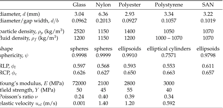
Table 2.3. Random packing volume fractions for the currently used particles found by experimental measurement and calculated using the sphericity.

Property Glass Nylon Polyester Polystyrene SAN

Size d(mm) 3.04 6.36 2.93 3.34 3.22

d/b 0.0962 0.2013 0.0927 0.1057 0.1019

Sphericity

ψ 0.9998 0.9999 0.9910 0.7571 0.9798

cylindrical,ψc 0.8736 0.8736 0.8690 0.8528 0.8658

disk,ψd 0.8244 0.8254 0.8701 0.8356 0.8648

RLP,φl

measured 0.597 0.568 0.593 0.553 0.611

calculated 0.5844 0.5844 0.5883 0.5551 0.5898

error 2.1% 2.9% 0.8% 0.4% 3.5%

RCP,φc

measured 0.626 0.627 0.650 0.663 0.657

calculated 0.6370 0.637 0.6500 0.6552 0.6524

error 1.8% 1.6% 0.0% 1.2% 0.7%

(54)

fraction can also be calculated from equation (2.6) usingφc,∞ = 0.648(based on the

set-tling model of O’Hern et al. (2002)) andφl,∞ = 0.584. These calculated packing fractions

are shown in Table 2.3 accompanied by the error between the calculated and experimen-tally measured value. The average error for all particles is 1.5%.

2.3.2 Previously reported experiments

In previously reported experiments, researchers published the particle sizes or size distri-butions and the random close-packing volume fraction, which was either experimentally determined or estimated. The random loose-packing volume fraction was often not re-ported. As it is the hypothesis of this thesis that the random loose-packing volume fraction corresponds to a transition in the effective viscosity (as discussed in subsection 2.1.1) this volume fraction must be determined.

In order to estimate the random loose-packing volume fraction, the random close-packing volume fraction is used with the assumption that all of the reported particles are nearly spherical such that the equations outlined in subsection 2.2.5 can be used. The gen-eral agreement between the calculated and measured values shown in Table 2.3 reinforces the choice of this method for determining the RLP. Values for the random packing fractions are summarized in Table 2.4 and outlined in detail below:

Table 2.4. Previous experiments of non-Brownian shear flows

Experiments Solid d (mm) φ φc φl

Bagnold (1954) 50% paraffin &

lead stearate 1.32 0.134–0.623 0.637 0.60

Savage and

McKeown (1983) polystyrene

0.97

0.429–0.570

0.642 0.590

1.24 0.644 0.591

1.78 0.641 0.590

Hanes and Inman

(1985) glass beads

1.1 0.55–0.58 0.64 0.544

1.85 0.49–0.5 0.55 0.441

Acrivos et al. (1994) PMMA 0.1375 0.20–0.30 0.58a 0.58a

acrylic 0.0905 0.20–0.50

Prasad and Kytömaa

(1995) acrylic 3.175 0.493–0.561 0.565 0.512

(55)

• Bagnold (1954): In his paper, Bagnold normalized the volume fraction by the the-oretical limit of φ = 0.74 for perfectly ordered spheres. In a later paper, Bagnold measured the “fluidity” packing fraction – below which the residual shear resistance at zero shear rate disappears – asφ = 0.60 (Bagnold 1966). In later analyses of his work, the RCP volume fraction has been taken as either the fluidity volume frac-tion (Savage and McKeown 1983) or asφ= 0.65(Hanes and Inman 1985). As fluidity should correspond more closely to (but is not necessarily) the RLP volume fraction, Bagnold’s reported value ofφ = 0.60 is used as the random loose-packing volume fraction. As no RCP value was reported, the theoretical value (φc= 0.637) was used

for the close-packing volume fraction (Finney 1970).

• Savage and McKeown (1983): Using the reported values for the RCP, the RLP was

estimated for nearly spherical particles based on the 10th-order extrapolation using

φc,∞= 0.637andφl,∞ = 0.584. Values ofφl= 0.590,0.591, and0.590were obtained

for thed= 0.97,1.24,1.78mm particles, respectively.

• Hanes and Inman (1985): In the experiment by Hanes and Inman, non-neutrally

buoy-ant particles were confined to an annular region, the top plate of which was allowed to move axially, but was subjected to a non-zero load during the experiment. Due to this geometry, the measured volume fractions were all confined between φl and φc. Hanes and Inman report the RCP volume fractions, but do not report the RLP

volume fractions. These values were estimated using the 10th-order extrapolation using φc,∞ = 0.637andφl,∞ = 0.584. For the d = 1.1 and1.85mm particles, the

extrapolation yielded values ofφl= 0.544and0.441. Both of these values are below

the minimum volume fraction tested, as expected.

• Acrivos et al. (1994): In their 1994 paper, Acrivos et al. did not determine φc

inde-pendently, but used the value obtained from a previous experiment. In Leighton and Acrivos (1987), using46µm polystyrene beads,φcwas determined as a fitting

param-eter to be 0.58. In their paper, Acrivos et al. claimed that this value is consistent with their results, but for two different types of particles (137.5µm PMMA and90.5µm acrylic). With no other information with which to make a determination, the value of 0.58 as reported in Leighton and Acrivos (1987) is used asφcandφl. This value is

(56)

RCP (Table 2.1).

• Prasad and Kytömaa (1995): In the experiments by Prasad and Kytömaa, the RCP

volume fraction was reported as φc = 0.565. This reported value differs

signifi-cantly from other values for RCP (Table 2.1), but may be due to the large particles (d/b= 0.294). If the same reduction was present in RLP – as expected using the data presented in Figure 2.5 for the influence on packing fraction on diameter ratio – a value ofφl= 0.512is appropriate. This value is consistent with the transition shown

in effective viscosity for their data.

2.4

Summary

The volume fraction of solids, φ, can dramatically change the effective viscosity of the liquid-solid flow. The random close-packed (RCP) volume fractionφcrepresents the

vol-ume fraction at which no more compaction occurs. At this volvol-ume fraction, the mixture is unable to shear without requiring deformation of either the particles or the surrounding cylinder walls. The random loose-packed (RLP) volume fractionφlis the volume fraction

where each particle is in contact with at least one adjacent particle. This volume fraction is the volume fraction obtained when shearing particles are allowed to freely dilate and represents the transition between an advective dominated diffusion and collision domi-nated diffusion. Aboveφl, as the volume fraction approachesφc, the effective viscosity is

expected to asymptotically increase. Below φl, a different