Improving predictability of the future by grasping probability less tightly

(1)

The London School of Economics and Political Science

Improving Predictability of the Future by

Grasping Probability Less Tightly

Edward Wheatcroft

A thesis submitted to the Department of Statistics

of the London School of Economics for the degree of Doctor of Philosophy.

(2)

Declaration

I certify that the thesis I have presented for examination for the MPhil/PhD degree of the London School of Economics and Political Science is solely my own work other than where I have clearly indicated that it is the work of others (in which case the extent of any work carried out jointly by me and any other person is clearly identied in it).

The copyright of this thesis rests with the author. Quotation from it is permitted, provided that full acknowledgement is made. This thesis may not be reproduced without my prior written consent.

I warrant that this authorisation does not, to the best of my belief, infringe the rights of any third party.

I declare that my thesis consists of 40,891 words.

(3)

Abstract

In the last 30 years, whilst there has been an explosion in our ability to make quan-tative predictions, less progress has been made in terms of building useful forecasts to aid decision support. In most real world systems, single point forecasts are fun-damentally limited because they only simulate a single scenario and thus do not account for observational uncertainty. Ensemble forecasts aim to account for this uncertainty but are of limited use since it is unclear how they should be interpreted. Building probabilistic forecast densities is a theoretically sound approach with an end result that is easy to interpret for decision makers; it is not clear how to imple-ment this approach given finite ensemble sizes and structurally imperfect models. This thesis explores methods that aid the interpretation of model simulations into predictions of the real world. This includes evaluation of forecasts, evaluation of the models used to make forecasts and the evaluation of the techniques used to interpret ensembles of simulations as forecasts. Bayes theorem is a fundamental relationship used to update a prior probability of the occurence of some event given new infor-mation. Under the assumption that each of the probabilities in Bayes theorem are perfect, it can be shown to make optimal use of the information available. Bayes theorem can also be applied to probability density functions and thus updating some previously constructed forecast density with a new one can be expected to improve forecast skill, as long as each forecast density gives a good representation of the uncertainty at that point in time. The relevance of the probability calculus, how-ever, is in doubt when the forecasting system is imperfect, as is always the case in real world systems. Taking the view that we wish to maximise the logarithm of the probability density placed on the outcome, two new approaches to the combination of forecast densities formed at different lead times are introduced and shown to be informative even in the imperfect model scenario, that is a case where the Bayesian approach is shown to fail.

(4)

Acknowledgements

I would like to thank my supervisor Professor Leonard Smith for his invaluable contribution to the work in this thesis. His enthusiasm and wisdom has been an endless source of motivation and inspiration throughout.

I would also like to thank all members of CATS for their support and friendship over the years and making my time at LSE a thoroughly rewarding and enjoyable experience.

(5)

‘All models are wrong, but some are useful.’

George E. P. Box

(6)

List of Tables

3.1 The ACC of the forecastsx1, .., xn, the slope parameter b from fitting

a regression of y1, .., yn on x1, .., xn, the error of the original forecast

xn and the error of the calibrated forecast ˜xn for different values ofn. 68

5.1 Summary of the origins of the methods used in this chapter. . . 95 5.2 The optimised values of the blending parameter α and the kernel

width σ, the optimised mean ignorance score over the training set and the mean ignorance over the test set from applying simple kernel dressing to the ensembles in experiment 5.A formed using a perfect model of the Lorenz ’63 system. . . 101 5.3 Mean ignorance scores relative to simple kernel dressing of forecast

densities formed from the test set of experiment 5.A usingK groups kernel dressing for different values of K. Also shown are resampling intervals of the mean relative ignorance. Since, for the first 6 values of K considered, zero does not fall into the resampling intervals, K

groups kernel dressing yields significantly more skillful forecasts than simple kernel dressing for these values of K. . . 112

(13)

LIST OF TABLES xii

5.4 Mean ignorance scores relative to simple kernel dressing of the fore-cast densities formed from the test set of experiment 5.A using fixed window kernel dressing for different values of M. Also shown are 95 percent resampling intervals of the mean relative ignorance in each case. Since zero does not fall into these intervals, a significant im-provement is made over simple kernel dressing for all values of M

considered except M = 16. The most effective value of M out of

those considered appears to be 256. . . 121

5.5 The optimised parameter values, the minimised mean ignorance over the training set and the mean ignorance over the test set obtained from applying dynamic kernel dressing to the ensemble-outcome pairs in experiment 5.A. . . 123

6.1 Summary of the origins of methods used in this chapter. . . 144

6.2 Weighting parameters of sequential blending for the Lorenz ’63 PMS in experiment 6.B. . . 168

7.1 Climatological standard deviations of the the PST system defined in appendix A.2.4 . . . 178

7.2 Results of applying PDA with and without rescaling the observations first. Values in brackets represent 95 percent resampling intervals. . . 182

8.1 Mean boosted probability times using each combination of ensem-ble formation scheme and kernel dressing method in experiment 8.C. Standard deviations are shown in brackets in each case. . . 202

B.1 Details of experiment 4.A . . . 235

B.2 Details of experiment 4.B . . . 236

B.3 Details of experiment 4.C . . . 236

(14)

B.8 Initial conditions for the system trajectory in experiment 7.B shown in figure 7.2 and 7.3. . . 239

B.14 Details of experiment 8.D . . . 242

B.15 Details of experiment 8.E . . . 242

B.16 Details of experiment 8.F . . . 243

(15)

List of Figures

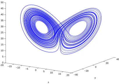
2.1 The Lorenz attractor with the traditional parameter values defined in appendix A.2.1. In the long term, all system states will lie on the system attractor. . . 16 2.2 Two indistinguishable states on the Ikeda map attractor. The red

cross represents the true state x0 whilst the red circle surrounding

it represents the bound of the observational uncertainty, that is the area in which an observation can fall. The green cross and the circle surrounding it represents another state y0 and its bound of

uncer-tainty. Since the observations0, represented with the red star, lies in

the overlapping region of the two uncertainty bounds, x0 and y0 are

indistinguishable. . . 23 2.3 States on the Ikeda attractor coloured according to whether they are

distinguishable or indistinguishable from the true state x0 given an

observation s0. x0 and s0 are represented with a red cross and a red

star respectively. States that are indistinguishable from the true state are coloured green. . . 24 2.4 Sets of indistinguishable states (coloured green) at time t = 0 given

the number of observations stated in each panel. As more past obser-vations are taken into account, the number of indistinguishable states diminishes. . . 26

(16)

LIST OF FIGURES xv

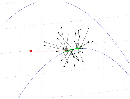
2.5 A demonstration of how PDA ensembles are formed for a perfect model of the logistic map. The blue line represents sets of 3 consec-utive states that are consistent with the model. The blue diagonal cross represents the final 3 points of the system trajectory which con-sists of a total of 16 time steps (the first 13 steps are not shown on the plot). The red point represents the final three observations (the point where PDA starts) which are assimilated to obtain the reference pseudo-orbit represented with the red cross. The black points are the result of adding random perturbations to the reference pseudo-orbit which are assimilated using PDA to obtain the green points which form the final initial condition ensemble. A close up view of the points is shown in figure 2.6. . . 32 2.6 A close up view of the points in figure 2.5. . . 33

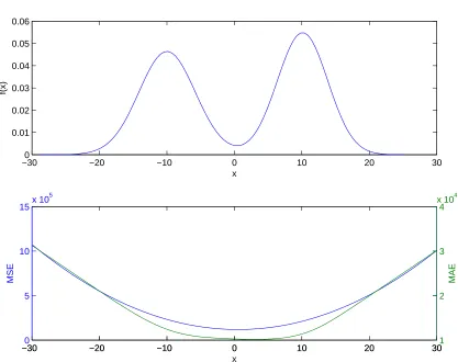
3.1 Upper panel: A system density in which the mean, median and mode all differ. Lower panel: The mean squared error (blue line corre-sponding to the left y axis) and the mean absolute error (green line corresponding to the right y axis) between 1024 random draws from the system density in the upper panel and the forecast values on the

x axis. In this case, both measures favour forecasts in which there is only low system density. . . 50 3.2 Upper panel: A time series of outcomes (black points) formed using

equation 3.11 withσ = 0.4 where the climatological meanµ(t), repre-sented with the black line, is governed by equation 3.13. Lower panel: The same time series linearly detrended. Linearly detrending fails to remove all of the effects of changes in the climatological mean. . . 58 3.3 The mean of the correlation coefficent between estimated anomalies

(17)

LIST OF FIGURES xvi

3.4 Scatter plot of the standard deviation of daily temperatures against the ACC of our artificial forecasts for each month in the CET record. The blue line shows the expected ACC as a function of the standard deviation of the outcomes as described in equation 3.19. Although the expected forecast error remains constant, the ACC tends to increase as a function of the standard deviation of the observed temperatures. 63 3.5 A scenario in which the relationship between a set of 16 forecasts and

outcomes is governed according to the behaviour of a logarithmic spiral. The x and y coordinates of the blue crosses represent the forecast values and the outcomes respectively. The red crosses, linked to the blue crosses, represent forecasts calibrated using linear regression. 66

4.1 Two shadowing trajectories of a one dimensional flow. The red cir-cles represent ’noisy’ observations whilst the red crosses represent the bounds of the noise. If a trajectory falls within the bounds of the noise, it is said to shadow the observation. The trajectories coloured blue and green, shown as solid when they are considered to shadow and dashed thereafter, shadow for 7 and 3 time steps respectively. . . 74 4.2 Upper panel: Mean shadowing lengths with 95 percent bootstrap

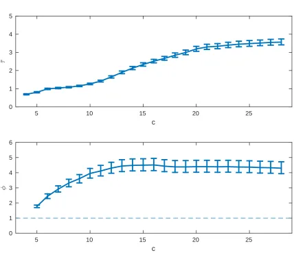
re-sampling intervals for different values of the imperfection parameterc

(18)

LIST OF FIGURES xvii

4.3 For experiment 4.B. Top left: Mean shadowing times of ensembles formed using inverse noise (blue), PDA with an assimilation window of 8 (red) time steps and PDA with an assimilation window of 16 time steps (yellow) as a function of ensemble size. Top right: Mean differences between shadowing times of ensembles formed using PDA with an assimilation window of 8 steps and inverse noise (blue) and PDA with assimilation windows of 16 and 8 time steps (red) as a function of ensemble size with 95% resampling intervals. Bottom: ensemble shadowing ratios between PDA with a window of 8 time steps and inverse noise (blue) and PDA with windows of 16 and 8 time steps (red) with 95% resampling intervals of the proportion as a function of ensemble size. For each given ensemble size, both the mean ensemble shadowing time and the shadowing ratio suggest that PDA performs better, on average, than inverse noise. Doubling the assimilation window, however, appears to make little difference to the performance of PDA in this case. . . 85 4.4 As a function of lead time: the mean ignorance score of forecast

den-sities formed using forecasting system A (red line, left axis) with 95 percent resampling intervals, the blending parameter α (blue line, right axis) of forecasting system A and the proportion of forecast densities (with 90 percent confidence intervals) that boost probability for forecasting system A (solid green line, right axis) and B (dashed green line, right axis). Here, boosted probability identifies how, al-though the forecast densities formed using forecasting system B per-form worse than forecasting system A in terms of the mean ignorance score, those formed using the former can sometimes be informative, whilst, for the latter, when α= 0, this can never be the case. . . 89

(19)

LIST OF FIGURES xviii

5.2 Two sets of ensemble members on the attractor of the Lorenz ’63 system evolved forward 3.2 days in Lorenz time. The ensemble mem-bers coloured green evolve over a section of the attractor in which there is little uncertainty and thus stay close together. The ensemble members coloured in red, on the other hand, evolve over a section of the attractor on which there is significant uncertainty as to whether a trajectory will remain on the same wing or move to the other and thus the ensemble standard deviation is much larger. . . 99 5.3 Kernel density estimates from samples of size 256 drawn from the

logistic distribution with, top left: s = 1 and σ = 0.6, top right:

s = 5 and σ = 0.6. Bottom left: s = 1 and σ = 2.5, bottom right:

s = 5 and σ = 2.5. In each case, the dashed line represents the true distribution from which the sample was drawn and the green line represents the estimated distribution. The black crosses at the bottom represent the positions of the sample members. Each of the underlying distributions can be estimated well with a good choice of kernel width but this cannot be done when the kernel widths are constrained to be equal. . . 100 5.4 Histogram of the ignorance scores of forecast densities formed from

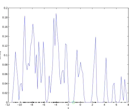
ensembles in the test set in experiment 5.A using simple kernel dress-ing. Although most of the forecasts perform much better than clima-tology, some have very high ignorance scores. . . 103 5.5 The forecast density with the worst ignorance score of all those formed

(20)

LIST OF FIGURES xix

5.6 The forecast density formed using simple kernel dressing from the ensemble with the highest standard deviation of all those in the test set in experiment 5.A. The ensemble and the outcome are represented by the black crosses and the green circle respectively. As in figure 5.5, it appears that the kernel width is too small. In this case, however, the outcome happens to lie much closer to the nearest ensemble member and hence the ignorance score is much better. . . 106 5.7 Scatter plot of the standard deviation of ensembles in the test set

against the ignorance of the forecast densities formed using simple kernel dressing in experiment 5.A. Ensembles with high standard de-viation are more likely to yield forecast densities that perform worse than climatology. . . 107 5.8 The mean ignorance as a function of the kernel width for the entire

training set (top),G1(bottom left) andG2(bottom right) inKgroups

kernel dressing for the case when K = 2 for the ensemble-outcome pairs defined in experiment 5.A. In each case, the optimal kernel widths, represented with black vertical lines, are different. . . 110 5.9 Top: The standard deviation of ensembles in the training set (short

dark blue lines) of experiment 5.A along with lines indicating the boundaries that determine which set of parameters should be used to dress a new ensemble for K = 2 (light blue), K = 4 (green) and

K = 8 (red) in theK groups method. Bottom: Kernel widths chosen to dress a new ensemble with a given standard deviation for K = 2 (light blue), K = 4 (green) and K = 8 (red). . . 111 5.10 Top: Fitted kernel widths for ensembles in the test set of experiment

5.A that fall into each group usingKgroups kernel dressing withK = 16 (red circles) and simple kernel dressing (blue crosses). Bottom: Mean ignorance of forecast densities formed from ensembles that fall into each group usingKgroups method (red circles) and simple kernel dressing (blue crosses). The increased skill achieved from using K

(21)

LIST OF FIGURES xx

5.11 The optimised mean ignorance over the training set (blue), the mean ignorance obtained using 2 fold cross validation (green) and the mean ignorance over the test set (red) as a function ofK for the ensemble-outcome pairs defined in experiment 5.A. Here, it is clear how 2 fold cross validation fails to identify the optimal number of groups. . . 116 5.12 An example of how the subset of the training set is selected in fixed

window kernel dressing for the case M = 32. The long black line represents the standard deviation of the ensemble to be dressed while the smaller lines represent the standard deviation of the ensembles in the training set. Those that are coloured red represent the ensemble-outcome pairs over which the parameter values are optimised. . . 118 5.13 The kernel width used to dress an ensemble with a given standard

deviation for M = 16 (blue), M = 128 (green) and M = 1024 (red) using fixed window kernel dressing with the ensemble outcome pairs defined in experiment 5.A. . . 120 5.14 Forecast densities formed using dynamic (green) and simple (blue)

kernel dressing from the ensemble in the test set of experiment 5.A which produces the highest ignorance score when simple kernel dress-ing is applied (as shown in figure 5.5). The black crosses along the

x axis show the positions of the ensemble members and the green circle the position of the outcome. By taking account of the ensemble standard deviation, dynamic kernel dressing is able to apply a larger kernel width and hence yield a more informative forecast density. . . 124 5.15 Forecast densities formed using dynamic (green) and simple (blue)

kernel dressing from the ensemble in the test set of experiment 5.A with the lowest standard deviation. The black crosses along the x

(22)

LIST OF FIGURES xxi

5.16 Scatter plot of the ignorance of forecast densities formed from the test set of experiment 5.A using simple and dynamic kernel dressing. Each point is coloured according to its ensemble standard deviation with warmer colours indicating those with high standard deviation. The blue line indicates the points at which the ignorance of both methods would be equal. It is clear that most of the improvement in skill yielded from dynamic kernel dressing comes from ensembles with relatively low or relatively high standard deviation since these points are much more likely to lie above the blue line. . . 127 5.17 The mean ignorance of forecast densities formed from 8 member

en-sembles using simple (blue solid lines) and dynamic (green solid lines) kernel dressing averaged over 64 repeats for each training set size. The error bars represent 90 percent bootstrap resampling intervals. Using the same colour scheme, the dashed lines show the mean optimised mean ignorance for each training set size. For ensembles of this size, dynamic kernel dressing yields a significant improvement in ignorance even when the training set is very small. . . 131 5.18 The mean ignorance of forecast densities formed from 64 member

en-sembles using simple kernel dressing (blue solid lines) and dynamic kernel dressing (green solid lines) averaged over 64 repeats for each training set size. The error bars represent 90 percent bootstrap inter-vals. Using the same colour scheme, the dashed lines show the mean optimised ignorance for each training set size. Dynamic kernel dress-ing yields a significant improvement in forecast skill for traindress-ing sets consisting of 32 ensemble-outcome pairs and more. For the smallest training set sizes, there is still some improvement but this difference is not significant for this ensemble size. . . 132 5.19 The kernel width that optimises the KL divergence (red dots), the

(23)

LIST OF FIGURES xxii

5.20 Forecast densities formed from the ensembles in the test set with the largest (upper panel) and smallest (lower panel) standard deviation using simple (blue) and dynamic (green) kernel dressing. Also shown is the forecast density obtained by applying the kernel width that minimises the KL divergence (red). The black dashed line represents the system density from which both the ensemble and outcome are drawn. In both cases, dynamic kernel dressing gets much closer to recovering the system density. . . 138 5.21 Top left:the mean ignorance score of forecast densities formed using

(24)

LIST OF FIGURES xxiii

6.1 The mean ignorance score, expressed relative to that of the standard method, of 8192 forecast densities formed using the naive method (green stars) on multiple lead time ensembles where 32 ensemble members were launched at a lead time of 96 hours and another 32 at 96 +h hours for different values of h. The error bars represent 95 percent resampling intervals of the mean relative ignorance. The dotted line represents the mean relative ignorance achieved by setting

h = 0 (i.e. doubling the ensemble size 96 hours ahead.) Since zero does not lie within the resampling intervals, when h takes a value of 54 hours or less, there is significant evidence that the naive method of combining forecast densities yields improved skill over the standard method. For larger values of h, there is no significant evidence of an improvement in skill whilst, for values of h of 78 hours and longer, there is significant evidence that the forecast densities perform worse on average than the standard method. . . 149 6.2 The same as figure 6.1 with the results of using the time-weighted

method added (red stars). Applying this approach results in skillful forecast densities from larger values of h. Unlike those formed using the naive method, forecast densities formed using the time-weighted method are never expected to perform worse than those formed using the standard method. . . 153 6.3 The results of applying the Pure Bayes method in the Lorenz ’63

(25)

LIST OF FIGURES xxiv

6.4 The results of applying the Pure Bayes method in the Lorenz ’63 per-fect model scenario of experiment 6.B. The black stars show the mean ignorance of the original forecasts whilst the blue lines show the mean ignorance using the Pure Bayes method where the starting point of each line indicates where the updating process was first applied. The colour of the points on the blue lines indicate whether the Pure Bayes method performs significantly worse than (red), better than (green) or not significantly different to (yellow) the original forecasts. In this scenario, in many cases, the Pure Bayes method yields significantly improved forecasts whilst using the climatology as a prior, on the other hand, appears to be counterproductive. . . 164 6.5 Mean ignorance scores of sequential blending expressed relative to

that of the standard method with 95 percent bootstrap resampling intervals of the mean in the Lorenz ’63 PMS. Since sequential blend-ing yields a lower mean ignorance score and the resamplblend-ing intervals do not contain zero, there is significant evidence that this approach performs better than the standard method in 8 out of 9 lead times considered. . . 167 6.6 Mean ignorance scores of sequential blending expressed relative to

(26)

LIST OF FIGURES xxv

7.1 Top panel: Mean shadowing length of model trajectories formed using PDA with an exact (blue) and an approximate (red) Jacobian as a function of the assimilation window. The error bars represent 95% resampling intervals of the mean in each case. Since the means are so close, it is difficult to distinguish the lines. Middle panel: The mean pairwise difference between the shadowing lengths of model trajectories formed using PDA with an exact and an approximate Jacobian with 95% resampling intervals of the mean difference. Lower panel: Shadowing ratios of model trajectories formed using an exact and approximate Jacobian. The error bars represent 95% resampling intervals of the shadowing ratio. Since the mean difference between the shadowing lengths is not significantly different from zero and the shadowing ratio is not significantly different from 1, both measures suggest a lack of a difference between the performance of each approach.175 7.2 The results of assimilating using PDA without rescaling the variables

first. For each variable, the black lines are the true trajectory, the red dots the observations and the green lines are the analysis. Although PDA has found a pseudo-orbit that stays close to the observations of the x,y,X and Y variables, this is not the case for the Z variable. . . 179 7.3 The same as figure 7.2 but with the modified version of PDA in which

the variables are rescaled. This time, the pseudo-orbit stays close to the observations of all of the variables. . . 181 7.4 Points on the attractor of the R¨ossler map coloured according to the

(27)

LIST OF FIGURES xxvi

7.5 Top left panel:the mean length of the linear regime as a function of F. Top right: the mean shadowing lengths achieved using PDA (blue), 4DVAR (red) and when no data assimilation is used (orange) as a function of F. The error bars represent 95 percent resampling intervals of the mean. Bottom left: the mean difference in shadowing lengths between PDA and 4DVAR (green) and between 4DVAR and when no data assimilation is used (red) as a function ofF. The error bars represent 95 percent resampling intervals of the mean difference in shadowing length. Botttom right: Shadowing ratios between PDA and 4DVAR (green) and between 4DVAR and the observations (red) as a function of F. The error bars represent 95 percent resampling intervals of the shadowing ratio in each case. . . 187

8.1 The standard deviation (blue points) along with the mean (black solid line) and the median (black dashed line) standard deviation at each lead time of the ensembles in experiment 8.A. Although, on average, the standard deviation of the ensembles increases with lead time, there is significant variation at each one. . . 194 8.2 The mean ignorance scores of forecast densities formed using

sim-ple (blue) and dynamic (green) kernel dressing for the 10 different lead times in experiment 8.A. The error bars represent 95 percent bootstrap resampling intervals of the mean ignorance. At most lead times considered, dynamic kernel dressing yields more skillful forecast densities, on average, than simple kernel dressing. . . 195 8.3 The standard deviation (blue points) along with the mean (black

solid line) and the median (black dashed line) standard deviation of the ensembles at each lead time in experiment 8.B. Although, on average, the standard deviation of the ensembles increases with lead time, there is significant variation at each one. . . 197 8.4 The mean ignorance scores of forecast densities formed using simple

(28)

LIST OF FIGURES xxvii

8.5 Mean ignorance of forecast densities formed using dynamic kernel dressing relative to the ignorance of forecast densities formed using simple kernel dressing as a function of lead time for experiment 8.A (blue), in which ensembles are formed using an imperfect model of the Henon map, and experiment 8.B (red), in which ensembles are formed using an imperfect model of the Lorenz ’96 system. The fact that zero does not fall within the resampling bars suggests that dynamic kernel dressing performs significantly better than simple kernel dressing at many of the lead times considered in these two examples. . . 200 8.6 Proportion of instances in which probability is boosted as a function of

lead time using dynamic (solid lines) and simple (dashed lines) kernel dressing with inverse noise (blue) and PDA ensembles (red) on the ensembles formed from the perfect model of the Lorenz ’63 system in experiment 8.C. The error bars represent 95 percent confidence intervals of each proportion at a subset of lead times. . . 203 8.7 Top: The mean ignorance scores obtained by applying the Pure Bayes

(29)

LIST OF FIGURES xxviii

8.8 Top: The mean ignorance scores obtained by applying the Pure Bayes method (blue lines), the time-weighted method (red crosses) and se-quential blending (cyan diagonal crosses) for the perfect model of the Moore-Spiegel system in experiment 8.D. The black circles rep-resent the mean ignorance scores of the original forecast densities. Bottom left: The mean ignorance scores of the Pure Bayes method with coloured dots indicating whether the forecasts are significantly than (better), worse than (red) or not significantly different from (yellow) the original forecasts. Bottom right: Mean relative igno-rance scores between sequential blending and the original forecasts (blue), the time weighted method and the original forecasts (red) and the time weighted method and sequential blending (orange) with 95% resampling intervals of the mean difference. In this case, for shorter lead times, the Pure Bayes method tends to yield forecast densities that are significantly better than the original forecasts whilst at longer lead times they tend to be worse. Both the time weighted method and sequential blending are able to yield significantly improved forecasts for all but the two shortest lead times. . . 208 8.9 The mean proportion of ensemble members that shadow the

(30)

LIST OF FIGURES xxix

8.10 The mean proportion of ensemble members that shadow the observa-tions (blue line, left axis) and the mean ignorance score obtained by fitting Gaussian distributions with (magenta starred line, right axis) and without (red starred line, right axis) blending as a function of forecast lead time. The error bars represent 95% resampling intervals of the mean ignorance. Forecasts formed without blending only yield significant skill with respect to climatology up to 6 steps ahead whilst blending increases this time to 13 steps. . . 212 8.11 The mean proportion of ensemble members that shadow the

obser-vations (blue line, left axis), the mean ignorance score obtained by fitting Gaussian distributions with (magenta starred line, right axis) and without (red starred line, right axis) blending and the mean ig-norance score obtained using dynamic kernel dressing (green starred line, right axis) as a function of forecast lead time in experiment 8.E. The error bars represent 95% resampling intervals of the mean ig-norance. Dynamic kernel dressing makes no assumption about the underlying distribution and thus yields better forecast skill than the Gaussian approach. . . 213 8.12 The mean proportion of ensemble members that shadow the

obser-vations (blue line, left axis), the mean ignorance score obtained by fitting Gaussian distributions with (magenta starred line, right axis) and without (red starred line, right axis) blending and the mean ig-norance score obtained using dynamic kernel dressing (green starred line, right axis) as a function of forecast lead time in experiment 8.F. The error bars represent 95% resampling intervals of the mean igno-rance. For the first 9 lead times, the approach of fitting Gaussian distributions without blending yields forecast densities that perform significantly better than climatology. The fact that a small propor-tion of ensemble members shadow longer than this time suggests that informative forecast densities may be found. This is confirmed by the performance of the forecasts formed using dynamic kernel dressing which yield better skill than the climatology up to 15 steps ahead. . . 215

(31)

A.2 The Duffing map attractor with parameter values a= 2.75 andb = 0.2.226 A.3 The Ikeda map attractor with parameter valuesα= 6,β = 0.4,γ = 1

and u= 0.83. . . 227 A.4 The Lorenz attractor with parameter values ρ= 28, σ = 10 and β = 8₃ 229 A.5 The Moore Spiegel attractor with parameter values R = 100 and

T = 35. . . 230 A.6 The R¨ossler attractor with parameter valuesa = 0.1 and b= 0.1 and

c= 14. . . 234

(32)

Chapter 1

Introduction

It has long been desirable for human beings to make predictions of the future. Early attempts at predicting the weather are known to have been made by Aristotle in around 340 B.C. [158] whilst some suggest that important battles have been won or at least significantly shortened on the basis of successful weather predictions (Meteorologists successfully predicted a short break in the stormy conditions that were occurring as the allies were planning the D-Day landings which allowed the operation to go ahead [1]).

Although it was recognised early on that weather conditions in one area could some-times be used to inform prediction of future weather patterns in another, such meth-ods were severely limited due to the fact that communication, whether over land or by sea, was slow. This, however, changed with the invention of the electric tele-graph in 1835 which meant that weather conditions could be communicated almost instantaneously [138] and thus the modern era of weather forecasting began. After a major storm in 1859, which caused the loss of the Royal Charter, 15 land stations

(33)

2

were set up so that reports of the weather could be submitted to experts and hence prior warnings of gales could be made to ships at sea. Over time, more stations were set up so that regular weather predictions, based on the knowledge of experts, could be disseminated [62].

The origins of numerical weather prediction techniques can be traced back to the works of Lewis Fry Richardson who took the (now very widely used) approach of representing the natural processes of the atmosphere as a set of differential equations and solving them using a straightforward numerical integration technique [102]. He used his method to make forecasts of changes in the pressure and the wind at two points over central Europe. In practice, however, numerical integration was highly laborious and time consuming. It was not until the advent of computing that forecasts could be made quicker than real time. The first numerical simulations of weather forecasts were made in 1950 [24] whilst the first regular, and hence operational, forecasts were made in Sweden in 1954 [64]. Subsequently, operational numerical forecasts became operational in countries around the world. [64]

Although Richardson’s first forecast was inaccurate, this allowed him to identify some of the challenges of numerical weather forecasting. He found that calculat-ing useful estimates of the initial state of the atmosphere1 _{could be difficult. The}

implications of this were further demonstrated in 1963 when Ed Lorenz showed, using a simple 3 dimensional model, that two simulations of a system with slightly different initial conditions will quickly diverge from each other [99]. As a result, he suggested that informative point predictions of the future state of the atmosphere can only be made up to around two weeks ahead. The true initial state of the atmo-sphere can never be found due to measurement error. It therefore became clear that

1

(34)

3

a deterministic forecast does not adequately reflect this uncertainty. Epstein [45] recognised this and proposed a dynamical model to predict the mean and variance of the distribution of possible future states. Whilst such Monte Carlo approaches were shown to be useful, it was suggested by Leith [95] that adequate representa-tions of the future states of the atmosphere could only be made using multiple point forecasts with initial states sampled from the uncertainty in observations of the cur-rent state. Such techniques are known as ensemble forecasts. Ensemble forecasts were introduced operationally both by the European Centre for Medium and Mid Range Forecasting (ECMWF) [105] and by the National Centers for Environmental prediction (NCEP) [151] in 1992 and soon many other forecasting centres followed suit [33, 2]. Whilst the original aim was merely to obtain a measure of likely fore-cast error, this paved the way for the formation and dissemination of probabilistic forecasts, in which the future states of a system are represented with probabilities or probability density functions. Such forecasts are desirable since they communicate information regarding the uncertainty in a forecast.

Probabilistic forecasts are in widespread use in many fields. For example, in weather prediction, precipitation forecasts expressed as probabilities have long been dissem-inated to the public [113, 51] whilst much emphasis is placed on the creation of probabilistic forecast densities of continuous variables such as the temperature. In climatology, projections of the future state of the climate are almost always proba-bilistic in nature [116] whilst probaproba-bilistic forecasting techniques are used in areas as diverse as population forecasting [159], economics [20] and ecology [9].

(35)

4

is always limited since, in the real world, any model will contain structural errors and therefore can only be considered to approximate the processes inherent in the system.

In this thesis, we focus on the following four aspects of the forecasting process:

1. Initial state estimation

2. Ensemble formation

3. Forecast density formation

4. Forecast Evaluation

We now briefly describe these and the contributions made in this thesis to each.

Initial State Estimation

(36)

5

Ensemble Formation

Ensemble forecasts are formed by sampling additional states around an observation or a ‘best guess’ of the initial state to form a set of initial conditions and using the model to evolve them forward in time to form a set of distinct model simulations which reflect the uncertainty/sensitivity of that particular forecast. The approach taken to the sampling of the initial conditions, however, is important and can have a large effect on the quality of the final forecast density. Generally, initial states that are consistent both with the observation and the model dynamics can be expected to perform better than those that are consistent only with the observation [81]. In section 4.2.1 and 8.2, we compare the performance of two ensemble formation techniques both in the context of the performance of the raw ensembles and forecast densities derived from them.

Ensemble Interpretation

(37)

6

a similar level of dispersion [143, 146]. In chapter 5, however, we show that this can yield systematically inferior forecast densities when this is not the case. We propose two new approaches to kernel dressing and consider an existing approach in which the varying level of dispersion in a set of ensembles is accounted for. We demonstrate that taking such approaches can improve the performance of sets of forecast densities.

In weather forecasting, ensembles are usually launched every 6 or 12 hours. Often, when a new ensemble is launched, it is used to form a new forecast density and the previous ensemble and forecast density are discarded. In chapter 5, we inves-tigate whether the most recently launched ensemble can be combined with those previously launched to yield better forecast densities. Whilst one might have ex-pected a Bayesian approach to be appropriate in this setting, we demonstrate, using examples, that it can, in fact, be counterproductive. It appears that flaws in the forecasting system, including model error, violate the common assumptions under-lying Bayes theorem; otherwise that approach would be effective. We introduce two new approaches to the combination of ensembles launched at different lead times and demonstrate that they can be used to construct forecast densities that perform significantly better than those formed with ensembles launched at a single lead time, even when the model is imperfect.

Forecast Evaluation

(38)

7

scoring rule is extremely important since, if it fails to identify the best forecast, it is of little use. Scoring rules also play an important role in the formation of forecast densities. Given a slowly increasing forecast-outcome archive, it is common for kernel dressing to use an independent set of ensembles and outcomes, called a training set, to train a set of forecast system parameters to optimise the performance with respect to a scoring rule.

In this thesis, we propose alternative approaches to forecast evaluation. A forecast evaluation method is optimised when the forecast that yields its best possible score is found. For point forecasts, distance based measures such as the mean squared error and the mean absolute error say little about their value since they are often optimised by the mean or the median of the distribution from which the outcome is drawn even if the probability of drawing such values is low. In chapter 3, we show that attempting to apply another common approach to the evaluation of point forecasts, the anomaly correlation coefficient skill score [4, 112, 111] can be misleading in practice and therefore should be treated with caution. We discuss an approach to forecast evaluation called shadowing and, capitalising on this concept, introduce a new approach called shadowing ratios.

It is useful to be able to assess various aspects of the ensembles themselves separately from the forecast (density). This means they can be assessed independently of forecast density formation and other interpretation techniques. In section 4.2.1, we introduce a new approach to the evaluation of ensembles, called ensemble shadowing ratios, in which the length of time the best performing member of each ensemble stays close to the observations is compared.

(39)

1.1. Thesis Structure 8

In section 4.3.1, we introduce a broader view of evaluating the performance of sets of forecast densities, called boosted probability, in which the period of time into the future they can be considered to be more informative than the distribution of the long term behaviour of the system is measured. This is not intended as an alternative to scoring rules, rather that boosted probability can be used alongside such measures to inform a forecaster about properties of the distribution of such scores.

1.1

Thesis Structure

It should be noted that, although each the research questions relate to the prediction of nonlinear systems, this thesis can be considered a collection of papers related to this theme rather than tackling an overarching research question. This thesis is structured in the following way:

In chapter 2, we provide background information on the process of forecasting dy-namical systems and an overview of the steps involved. We focus on the individual steps of the forecasting framework, detailing the methods drawn upon in this the-sis. Whilst the presentation of some of the material is new, there are no novel contributions in chapter 2.

In chapter 3 we turn our attention to the evaluation of point forecasts. We re-view some shortcomings of common evaluation techniques before focusing on the anomaly correlation coefficient skill score (ACC). We argue that this measure should be treated with extreme caution and that a very specific set of assumptions should be satisfied for its deployment to be valid.

(40)

this thesis: point forecasts, which consist of a single estimate of the future and probabilistic forecast densities, which take the form of predictive probability density functions. In addition, we consider the evaluation of ensembles, which consist of multiple point forecasts initialised with slightly different values. We introduce a new approach to the evaluation of forecast trajectories, called shadowing ratios, which measures forecast performance based on the length of time forecast trajectories stay close to or ‘shadow’ a set of observations. We extend this approach to introduce a new method, called ensemble shadowing ratios, aimed at evaluating the performance of ensembles. Finally, we introduce a new approach to the evaluation of a sequence of forecast densities, called boosted probability, which provides an alternative view to regular methods of probabilistic forecast evaluation.

In chapter 5, we focus on the formation of forecast densities from ensembles. We show that, when there is significant variation in the dispersion of ensembles resulting from nonlinearities in the system, simple kernel dressing fails to provide useful fore-cast densities in some cases. We thus propose two new methods and apply another existing method aimed at correcting this problem, showing that each one tends to yield, on average, more informative forecast densities. We then show that, when the ensemble and the outcome are drawn from the same distribution, one particular approach which we refer to as dynamic kernel dressing, performs much better in terms of how closely forecast densities approximate this distribution.

(41)

approach can be improved upon by allowing ensembles launched at different times to be weighted differently. We call this approach the time-weighted method. We then investigate how forecast densities, rather than ensembles, launched at different lead times can be combined to yield improved forecast skill. The Bayesian approach is the correct way of combining sequentially formed probabilities. We show, however, that, in practice, the Bayesian approach is always likely to be sub-optimal due to the effects of model error and other imperfections in the forecasting system.

Finally, we introduce a new approach called sequential blending, which, like the time-weighted method, is shown to be effective in improving forecast skill, even when the model is imperfect. With this method, forecast densities are formed by sequentially updating forecasts by extending the blending approach introduced in [22].

In chapter 7, we perform three experiments, using the approach of shadowing ratios introduced in chapter 3, to make comparisons between data assimilation techniques. In the first, we compare the performance of an approach called Pseudo-orbit data as-similation (PDA) when the required gradient information required for the algorithm is known and when it is replaced with an approximation. In the second experiment we show how PDA can fail when there are large differences in the variability of the variables it is applied to. We show how the algorithm can be altered to allow for this variability and that its performance is improved as a result. In the third experiment, we make a direct comparison between the performance of PDA and another data assimilation technique, called 4DVAR, in an environment in which the level of non-linearity in the system is varied. We show that, the more nonlinear the system, the bigger the improvement that can be made by applying PDA rather than 4DVAR.

(42)

approaches introduced in the preceding chapters. First, we turn our attention back to dynamic kernel dressing. In chapter 4, we show that this approach is capable of improving the skill of forecast densities in the perfect model scenario. In this chapter, we demonstrate, using two different imperfect models, that this approach can also be found to improve forecast skill in the imperfect model scenario.

Next, we make use of the boosted probability approach introduced in chapter 3 to compare the performance of forecast densities formed using different ensemble and density formation techniques. We show that PDA can outperform another approach called inverse noise. Moreover, we show that the dynamic kernel dressing method introduced in chapter 5 can yield further improved forecast densities compared with simple kernel dressing.

We then demonstrate that the results found in chapter 6, in which different ap-proaches to combining forecasts are investigated, can also be found in a different dynamical system. We argue that this gives us confidence that our results are likely to apply more generally.

Finally, we demonstrate the link between shadowing and forecast skill. We show that the period of time in which an ensemble of forecast trajectories shadow the observations can indicate whether skillful forecast densities can be expected to be found. We demonstrate how this approach would lead us to look for better fore-cast density formation techniques in the case when our forefore-cast densities consist of Gaussian distributions.

(43)

Chapter 2

Background Theory

In this chapter, we describe background theory to the processes used in forecasting and some of the concepts capitalised upon in this thesis. This chapter contains no novel material beyond its presentation.

In section 2.1, we define forecasting and describe the fundamental differences be-tween point forecasts, ensembles and probabilistic forecasts. We then describe our forecasting framework, a series of steps that make up the forecasting process. Next, we explain the important distinction between two forecasting scenarios used in this thesis: the perfect model scenario [140, 40], in which the underlying system pro-cesses are understood perfectly by a forecaster, and the imperfect model scenario, in which the model contains some level of structural uncertainty.

In section 2.2, we describe the theory of indistinguishable states [140, 141] and explain how this leads to the conclusion that, in the presence of observational noise, the true initial state cannot be distinguished from other model states. This forms the basis of the argument that forecasts should take the form of probability density

(44)

2.1. Forecasting 13

functions rather than single values.

In section 2.3, we explain the need for current state estimation techniques, or data assimilation [161, 40, 48]. We explain how data assimilation can be expected to improve forecast performance. We then describe two particular data assimilation techniques, pseudo-orbit data assimilation [80, 82, 41, 40] and 4DVAR [67, 68, 125], the performance of which we compare in chapter 7.

In section 2.4, we describe some of the methods used in the formation of probabilistic forecasts. We explain the rationale behind ensembles and describe two approaches to their formation. We then describe a number of approaches to ensemble interpre-tation in which ensembles are used to form forecast densities[129, 22].

2.1

Forecasting

Predicting the future evolution of any physical system is restricted by various types of uncertainty [99, 141]. To make predictions of future states, we attempt to build mathematical models of the underlying behaviour of a system. Since the complex rules of nature can never be understood perfectly, however, our models can only approximate the processes inherent in a system. Nevertheless, provided the model reproduces at least some of the key processes, we can often gain some understanding of how states may evolve. This process is called forecasting [10].

2.1.1

Dynamical Systems

Adynamical system is a set of rules governing the time dependence of a set ofstates x _∈ Sd _{in a geometric space where} xt is the state of the system at time t and Sd

(45)

2.1. Forecasting 14

system are called the dynamics. A dynamical system can be written in the form

xt = Ft(x0), where F denotes the dynamics of the system. x0 is called the initial

state or initial condition of the system.

Dynamical systems can be divided into two different types, stochastic and deter-ministic. In deterministic systems, a state and the dynamics define all future states unambiguously whilst stochastic systems include some random element in the dy-namics which means that two trajectories with different initial conditions can evolve differently over time. We consider only deterministic dynamical systems. Through-out this thesis, we assume that the model and the system share the same state space thereby avoiding issues of subtractability [100, 142].

2.1.2

Maps and flows

Dynamical systems can evolve either in discrete or continuous time. A system that evolves in discrete time is called a map and is defined by

xi+1 =F(xi), (2.1)

where i _∈ Z_{. The dynamics} _F _{govern the evolution from one discrete time step to}

the next. A dynamical system that evolves in continuous time is called a flow and is usually described by a set of ordinary differential equations in the form

dx(t)

dt =F(x), (2.2)

defined for all t _∈ R _{giving an unbroken continuous trajectory} xt for t ∈ (0, T).

(46)

2.1. Forecasting 15

a 4th order Runge-Kutta [91] integration scheme to define the system.

2.1.3

System-model pairs

Prediction of dynamical systems requires a forecasting model. A model attempts to give a mathematical description F, called the model dynamics, of the system dynamics F˜. Since it is impossible to perfectly describe the complex laws of nature, in real world forecasting problems, F and ˜F are necessarily distinct. We refer to the pair of dynamical systems governed by ˜F and F as a system-model pair. Details of the system-model pairs used in this thesis can be found in appendix B. An observation of a forecasted system state is called an outcome. We refer to a set of forecasts and corresponding outcomes as a forecast-outcome archive.

2.1.4

Chaos

Many real world dynamical systems are highly sensitive to initial condition uncer-tainty. This sensitivity is known aschaos [99] and is most famously known to occur in weather and climate but is also claimed to exist in a diverse set of fields such as psychology [72], economics [86] and ecology [104]. A common description of chaos, coined by Edward Lorenz, is that ‘the flap of a butterfly’s wings in Brazil can cause a tornado in Texas’ [43], the implication being that a small and seemingly insignifi-cant difference in the initial condition can lead to large differences later on. Chaos makes the task of prediction more difficult even when the model and the system dynamics are identical since small errors in the initial conditions will eventually

(47)

2.1. Forecasting 16

−20 ₋₁₅

−10 ₋₅

0 ₅

10 ₁₅

20 −40

−20 0

20

40 0

5 10 15 20 25 30 35 40 45 50

y

x

[image:47.595.126.535.160.448.2]

z

Figure 2.1: The Lorenz attractor with the traditional parameter values defined in appendix A.2.1. In the long term, all system states will lie on the system attractor.

Initial states of dynamical systems will tend to evolve over time towards a set of states called an attracting set. The collection of states in the attracting set is called the attractor. States that do not lie within the attracting set are called transient

(48)

2.1. Forecasting 17

2.1.5

Point and Probabilistic forecasting

Forecasts can either consist of single values or be probabilistic in nature. For ex-ample, a forecaster might predict rain tomorrow or that the temperature will be 27 degrees Celsius. A point is defined as a particular single state. A forecast consisting of a single point is called apoint forecast. Probabilistic forecasts, on the other hand, assign probabilities to different outcomes. For example, a forecaster might estimate a 90 percent chance of rain. Probabilistic forecasts of continuous variables consist of a probability density function called a forecast density.

2.1.6

Forecasting framework

The process of forecasting, as considered in this thesis, is conducted in a number of stages which we refer to as our forecasting framework. We briefly describe each of these stages below. A specific configuration of the forecasting framework is called a

forecasting system.

Collection of observations

(49)

2.1. Forecasting 18

the system1_.

Current state estimation

Current state estimation techniques combine sets of past and present observations with a model to attempt to find an improved estimate of the initial state. This process is calleddata assimilation [161, 40, 48]. Data assimilation techniques usually aim to find initial conditions that are consistent with both the observation(s) and the model dynamics. We discuss these in more detail in section 2.3.

Ensemble formation

Whilst data assimilation techniques can often be expected to find a more useful initial state for a model, we can never expect it to coincide with the underlying system state and thus some initial condition uncertainty will always be present. Therefore, instead of evolving a single model simulation, ensemble methods [96, 105, 151] attempt to account for initial condition uncertainty by running multiple simulations of the same model, each one with a slightly different initial condition. In point forecasting, this stage is usually omitted. We discuss ensemble formation in more detail in section 2.4.1.

Generation

At the generation stage, one or more initial conditions are evolved forward for a fixed period of time into the future called a lead time. If more than one initial condition is used, the resulting set of model trajectories is called an ensemble.

1

(50)

2.1. Forecasting 19

Removal of biases

Forecasts often contain inherent systematic biases which can be detected using pairs of forecasts and outcomes. These biases can either come from the limitations of the model or from variations within the area being forecast. For example, in weather forecasting, predictions of variables such as the temperature usually apply to fixed grid boxes on or above the Earth’s surface. Observed values are always likely to differ within each grid box depending on the topography of the local area and hence the forecast may consistently overestimate in some areas of the grid box and under-estimate in others. At this stage, removal of such biases is attempted using sets of historical forecasts and outcomes.

Ensemble Interpretation

At this stage, ensembles are used to form predictive forecast densities. This stage is omitted when the desired outcome is a point forecast. We discuss ensemble interpretation in more detail in section 2.4.3.

Forecast evaluation

(51)

2.1. Forecasting 20

2.1.7

Perfect and Imperfect model scenarios

In this thesis, we make use of both the perfect model scenario (PMS) and the imper-fect model scenario (IMS). These two concepts differ in the level of understanding a forecaster has of the underlying dynamics of a system. Both scenarios are defined below.

Imperfect model scenario

In the imperfect model scenario (IMS), the forecaster’s model provides only an ap-proximate representation of the underlying system dynamics. In fact, every real world forecasting problem falls into this category since, in practice, it is impossible for a model to reproduce all of nature’s processes perfectly. In the IMS, the existence of initial condition uncertainty is also assumed since real world measurements are always clouded in observational error, whether this be from finite precision measur-ing devices, roundmeasur-ing error, noise, human error, other, or a combination of these factors.

Perfect model scenario

(52)

2.2. Indistinguishable States 21

2.2

Indistinguishable States

With a perfect model of the system dynamics and a perfect initial condition, an ex-act point forecast of any future state of a deterministic system can be made. When an observation of the initial condition is clouded in measurement error, however, multiple model states will exist that are consistent with an observation given its error distribution and thus are indistinguishable from the true state. Such states are known as indistinguishable states [140, 141]. Under the perfect model scenario, evolving any of these states forward in time represents a plausible, but not neces-sarily equally likely, scenario of the future given the information contained in the observation.

We now describe the theory of indistinguishable states as introduced in [140] and [141]. Although we do not directly use indistinguishable states in this thesis, the the-ory provides useful justification for why probabilistic forecasts are more appropriate than point forecasts for nonlinear systems.

Let st represent an observation of the true state xt and let yt represent some other

state. Let the probability density function of the observational noise be ρ(.). The joint probability density function that an observation st renders xt and yt

indistin-guishable is thus given by

Z

ρ(st−xt)ρ(st−yt)dst. (2.3)

(53)

between the two states and z is the actual measurement error, define

g(b) =

Z

ρ(z)ρ(z₋b)dz (2.4) and normalise to obtain

q(b) = g(b)

g(0), (2.5)

such that q(b) is the probability that yt is indistinguishable from xt. Since q(0) = g(0)

g(0) = 1, a state is indistinguishable from itself with probability one.

The theory of indistinguishable states can be extended to a sequence of observed values. Given a time series of observations s=s0, s−1, s−2, ... of the true trajectory

x, the probability that x and a trajectory y are indistinguishable from each other is

Q(x,y) =Y

t_≤0

q(yt−xt) (2.6)

and hence if Q(x,y) = 0, the trajectories are distinguishable with probability one. Note that Q(x,y) is the probability that any set of observations will render two trajectories indistinguishable.

In practice, whilst the system state can only be known if no observational noise is present, it is, however, possible to find states that are indistinguishable from the true state. For two states to be indistinguishable, each one must be consistent with the observation. Since the true state xt is consistent with the observation st

with probability one, any state that is consistent with the observation must also be indistinguishable from the true state. The set of trajectories indistinguishable from

x is defined by

(54)

0.3 0.4 0.5 0.6 0.7 0.8 0.9 1 1.1 1.2

0.1 0.2 0.3 0.4 0.5 0.6 0.7 0.8 0.9

x

[image:54.595.158.499.111.383.2]

y

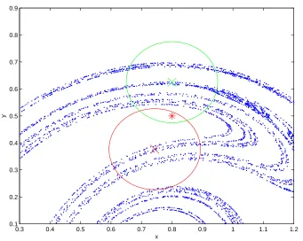
Figure 2.2: Two indistinguishable states on the Ikeda map attractor. The red cross represents the true state x0 whilst the red circle surrounding it represents the

bound of the observational uncertainty, that is the area in which an observation can fall. The green cross and the circle surrounding it represents another state y0

and its bound of uncertainty. Since the observation s0, represented with the red

star, lies in the overlapping region of the two uncertainty bounds, x0 and y0 are

indistinguishable.

An illustration of indistinguishable states is shown in figure 2.2. Here, the red cross represents a true statex0on the attractor of the Ikeda Map defined in appendix A.1.4

and the red circle surrounding it, the bound of the observational noise in which an observation ofx0 must fall. The green cross and the circle surrounding it represents

another system statey0 and the bound of its observational noise, that is the area in

which an observation of y0 must fall. The red star represents an observation s0 of

x0. Since the observation falls within the bounds of uncertainty of both states, and

hence could conceivably be an observation of either, y0 is indistinguishable from the

(55)

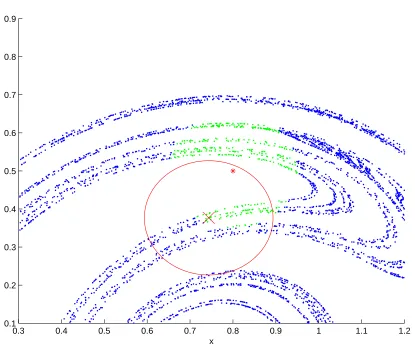
0.3 0.4 0.5 0.6 0.7 0.8 0.9 1 1.1 1.2 0.1

0.2 0.3 0.4 0.5 0.6 0.7 0.8 0.9

x

[image:55.595.125.540.103.450.2]

y

Figure 2.3: States on the Ikeda attractor coloured according to whether they are distinguishable or indistinguishable from the true state x0 given an observation s0.

x0 and s0 are represented with a red cross and a red star respectively. States that

are indistinguishable from the true state are coloured green.

The set of system states indistinguishable from the true state are coloured in green in figure 2.3 whilst those that are distinguishable are coloured blue. Note how the position of the observation influences the set of indistinguishable states.

Now, suppose that as well as the observation s0, a set of observations s−1, s−2, ...

of past states x₋1, x−2, ... is available. Each state at time t = 0 uniquely defines

a system trajectory stretching into the past. Suppose a state y0 is found that is

(56)

information, the two trajectories x and y cannot be distinguished. Now suppose that an observation from the previous time step s₋1 of x−1 is known. If y−1 is not

consistent with s₋1, the two states x−1 and y−1, and thus the two trajectories x

and y, are distinguishable. By considering extra observations from the past, the set of indistinguishable states can be reduced. This is demonstrated in figure 2.4. In the top left panel, states that are indistinguishable from the true state given only a single observation s0 are shown in green (as in figure 2.3). In the top right

panel, an observation from the previous time step s₋1 (not shown) is also taken

into account and the number of indistinguishable states is reduced. In the bottom left panel, observationss₋2,s−1 ands0 are taken into account whilst 4 observations

s₋3,s−2,s−1 ands0 are taken into account in the bottom right panel. As the number

of observations from the past increases, the number of trajectories that are consistent with x decreases.

2.2.1

Indistinguishable states and the case for probabilistic

forecasting

That taking more past observations into account reduces the range of indistinguish-able states might lead us to expect that as the number of past observations tends to

(57)

0.4 0.6 0.8 1 1.2 0.1 0.2 0.3 0.4 0.5 0.6 0.7 0.8 x y one step

0.4 0.6 0.8 1 1.2 0.1 0.2 0.3 0.4 0.5 0.6 0.7 0.8 x y two steps

0.4 0.6 0.8 1 1.2 0.1 0.2 0.3 0.4 0.5 0.6 0.7 0.8 x y three steps

[image:57.595.117.541.214.567.2]

0.4 0.6 0.8 1 1.2 0.1 0.2 0.3 0.4 0.5 0.6 0.7 0.8 x y four steps

(58)

2.3. Data Assimilation 27

point forecast initialised using one of these states can only be considered a single draw from the distribution of possible point forecasts given the set of observations and