Findings on a least hop (s) path using Bellman Ford algorithm

FINDINGS ON A LEAST HOP (s) PATH USING

BELLMAN-FORD ALGORITHM

NIK SHAHIDAH AFIFI MD TAUJUDDIN

MOHD HELMY ABD WAHAB

SITI ZARINA MOHD MUJI

ZARINA TUKIRAN

FIRST REGIONAL CONFERENCE ON

COMPUTATIONAL SCIENCE AND TECHNOLOGIES

2007

2 9 - 3 0 NOV 2007

V j '

i

Findings on A Least Hop(s) Path Using

Bellman-Ford Algorithm

Nik Shahidah Afifi

Bt. Md Taujuddin

Electronic Engineering, Universiti Tun Hussein O n n Malaysia (UTHM),

86400 Parit Raja, Batu Pahat, Johor,

MALAYSIA.

[email protected]

u.my

Mohd Helmy Abd

Wahab

Faculty of Electrical and Electronic Engineering, Universiti Tun Hussein O n n Malaysia (UTHM),

86400 Parit Raja, Batu Pahat, Johor,

MALAYSIA,

helmy

@uthm.edu.my

Siti Zarina Mohd

Muji

Faculty of Electrical and Electronic Engineering, Universiti T u n Hussein Onn Malaysia (UTHM),

86400 Parit Raja, Batu Pahat, Johor,

MALAYSIA,

szarina

@uthm.edu.my

Zarina Tukiran

Electronic Engineering, Universiti Tun Hussein O n n Malaysia (UTHM),

86400 Parit Raja, Batu Pahat, Johor,

MALAYSIA.

[email protected]

A B S T R A C T

As one of the most challenging problems in the next generation high-speed network constrain on service on routing. Bellman-Ford routing algorithm is one of the approach techniques being used to provide best strategy for QoS routing problems. This paper present the powerful of Bellman-Ford in solving most multiple constrained routing problems arise in the network. The discussions also highlight the application, advantages, and potential problems of the Bellman Ford as well as comparison with Dijikstra routing algorithm.

Keyword: Bellman-Ford Algorithm, Internet routing, shortest path.

I N T R O D U C T I O N

The classic Bellman-Ford algorithm that solves the single-source shortest path (SSSP) problem in network has been widely used and studied for over 35 years (Kolliopoulos and Stein, 1998).

Normally, when the diagram was given, the Bellman-Ford algorithm will find the shortest paths from a given source node subject to the constraints at most one link, then 2 most links and so on. The first step is to find all nodes 1 hop away, then find all nodes 2 hops away and followed by 3 hops and so on. The Iteration table is created based on the number of links. The routing table is formed based on the iteration table.

Routers that utilize these algorithm have to maintain the distance tables (which is a one-dimension array called "a vector"), which tell the distances and shortest path to sending packets to each node in the network. The information in the distance table is always updated by exchanging information with the neighboring nodes. The number or data in the table equals to all nodes in networks (excluded itself). The columns of table represent the directly attached neighbors whereas the rows represent all destinations in the network. Each data contains the path for sending packets to each destination in the network and distance or time to transmit on that path (also known as cost). The

measurements in this algorithm are the number of hops, latency and the number of outgoing packets.

The Bellman-Ford algorithm enables each node receives some information from one or more of its directly attached neighbors. The process of exchanging information will continue until no more information is exchanged between the neighborhoods. This algorithm does not require all of the nodes to operate in lock step with each other. Lock step can be defined that every time the nodes operate it does not need to use the same route.

There is a shortest path from s to any other vertex that does not contain a non-negative cycle (can be eliminated to produce a shorter path). The maximal number of edges in such a path with no cycles is Ivl-1, due to it can have at most / v / nodes on the path if there is no cycle. Therefore, it is enough to check paths of up to /v ]-l edges.

The Bellman-Ford algorithm uses d[u] as an upper bound on the distance d[u,v] from u to v. The algorithm progressively decreases an estimate d[v] on the weight of the shortest path from the source vertex s to each vertex v in V until it achieve the actual shortest-path. The algorithm returns Boolean TRUE if the given graph contains no negative cycles that are reachable from source vertex .v otherwise it returns Boolean FALSE.

Figure 1 below illustrates an example of opening of the Bellman Ford Algorithm.

BELLMAN-FORD (G, w, s)

INITIALIZE-SINGLE SOURCE (G, s) for each vertex i=l to V[G]-1 do

for each edge (u,v) in E[G] do RELAX (u,v,w)

For each edge (u,v) in E[G] do if d[u] + w(u,v) < d [v] then

return FALSE return TRUE

Figure 1. Opening Bellman Ford Algorithm

Let G be a weighted graph. The length (or weight) of a path P is the sum of the weights of the edges of P. If P consists of edges eO, el ,e2,...,ek-l then the length of P, w(P) is defined as

W

(P) = f > ( e , )

0)

The distance from a vertex v to a vertex u in G, d(v,u), is the length of a minimum length path (also called shortest path) from v to u, if such a path exists. The convention d(v,u) = +: if there is no path at all from v to u in G. Even if there is a path from v to u in G, the distance from v to u may not be defined, however, if there is a cycle in G whose total weight is negative. Any time edge weights are used to represent distances, it must be noted not to introduce any negative-weighted cycles.

Suppose that it is given a weighted graph G, and it is prompted to find the shortest path from some vertex v to each other vertex in G, viewing the weights on the edges as distances.

Theorem: Given a weighted directed graph , j r with n

vertices and m edges, and a vertex v _{of & , the} Bellman-Ford algorithm computes the distance from v

to all other vertices of G or determines that ^ contains a negative-weight cycle in O(nm) time.

2.0 B E L L M A N F O R D A L G O R I T H M

2.1 The Formal Bellman Ford

Algorithm

An initial assumption for distance-vector routing is each node knows the cost of the link of each of its directly connected neighbors. Next, every node sends a configured message to its directly connected neighbors containing its own distance table. Now, every node can learn and update its distance table with cost and next hops for all nodes network.

Repeat exchanging until no more information between the neighbors. Consider a node X that is interested in routing to destination Y via a directly attached neighbour Z. Node Xs distance table entry, Dx(Y,Z) is the sum of the cost of the direct-one hop link between X and Z, c(X,Z), plus neighboring Ts currently known minimum-cost path (shortest path) from itself (Z) to Y. That is Dx(Y,Z) = c(X,Z) + minw{Dz(Y,w)} where minw is taken over all the Zs.

The equation Dx(Y,Z) = c(X,Z) + minw{Dz(Y,w)} suggests that the form of neighbor-to-neighbor communication that will take place in the DV algorithm where each node must know the cost of each of its neighbors' minimum-cost path to each destination. Hence, whenever a node computes a new minimum cost to some destination, it must inform its neighbors of this new minimum cost.

2.2 The Simpler Bellman Ford

algorithm

The algorithm will send its routing table to all his neighbors whenever his link table changes. When we get a routing table from a neighbor on port P with link metric M:

1. Add L to each of the neighbor's metrics. 2. For each entry (D, P', M') in the updated neighbor's table:

2.1 If we do not have an entry for D, add (D, P, M') to my routing table.

2.2 if I have an entry for D with metric M", add (D, P, M') to my routing table ifM' < M"

if my routing table has changed, we send all the new entries to all my neighbors

3.0 H O W IT W O R K S

Example X

Figure 2. Network diagram with node 1 as source node

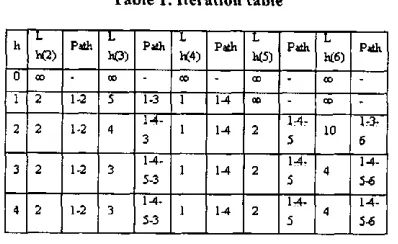
Table 1. Iteration table

h L K2) Path

L

Path 1 w Path

L ¥5) Path

L h(6) Path 0 CO - CO CO - CO - a>

-1 2 1-2 5 1-3 1 14 CO - CO

-2 -2 1-2 4

14-3 1 14 2 14-5 10

1-3-6

3 2 1-2 3

14-5-3 1 14 2 14-5 4

14-5-6

4 2 1-2 3

14-5-3 1 14 2 14-5 4

14-5-6

Table 1 show the iteration for Figure 2 with node 1 as source node.

Definition:

1. w (i,j) - link cost from i to j; w (ij) = 0, w (ij) = oo if the 2 nodes are not directly connected, w (ij) > 0 if the 2 nodes are directly connected

2. h = max number of links in a path at the current stage of the algorithm

3. L h(n) = cost of the least cost path from node 5 to node n under the constrain of no more than h links

4. Path = route to node n

For one number of links for hop 3, the path is 1-3 at cost 5. For two numbers of links for hop 3, the path is 1-4-3 at cost 4. The path 1-4-3 is chosen due to it gives a smaller cost. For three numbers of links for hop 3, the path is 1-4-5-3 at cost 3. The cost for this route is the smallest compared with the other routes therefore the shortest route is chosen. The same method is used for the other nodes.

Table 2. Routing table

Destination Rjoute Distance

2 1-2 2

3 1-4-5-3 3

4 1-4 1

5 1-4-5 2

6 1-4-5-6 4

Table 2 show the routing table for Figure 2.

Example 2

Bellman-Ford Algorithm able to find out the least cost paths from Node 1 to other nodes. In this case costs of paths shown are in two-way, for example, the cost of path 1-2 (path from Node 1 to Node 2) is the same as

the cost of path 2-1 (path from Node 2 to Node 1). Source node for this figure is node 1.

Iteration table for figure 3 can be represented in Table 3.

Table 3. Iteration table for example 2

h P i t B 1>3 Path3 C4 PatM DS b i PathS (i 99. 99 99. 99. 99. i a 1-2 99. 2 U 99 99

2 3 1-5 4 1 4 - 3 i 1-4 6 14-5 7 U - d 3 3 1-2 4 1-4-3 2 1 4 6 14-5 S 14-3-e 4 3 1-2 4 14-3 2 1-4 6 14-5 5 14-3-fi

Definition:

h - maximum number of links in a path at the current stage/step of the algorithm

D(n) - the cost of the least cost path from the source node to node n under the constraints of no more than h links.

At h=0, there is no path with maximum allowed link <= O.At h = l, paths 1-2 and 1-4 are with link < = 1 and hence added to the table. At h=2, we're allowed to consider paths with maximum link = 2, hence we'll check possible links from source node to each of other nodes in the network.

From 1 to 2, we found one more allowed link, 1-4-2, but it is with a higher cost (4) than path 1-2; hence we will stick with path 1 -2 and add it to the table.

From 1 to 3, two paths are found: 1-2-3 and 1-4-3. Path 1-4-3 has less cost (4) than path 1-2-3 (cost=6); hence path 1 -4-3 is added to the table.

From 1 to 5, there is only one path found which fits the constraint, link <=2: 1-4-5; hence we add this to the table.

From 1 to 6, there is only one path found which fits the constraint, link <=2: 1-4-6; hence we add this to the table.

as path 1-4-3-6 is with link =3, which violates the rules for current stage of having link <=2.

At h=3, we do the same as in h=2 while this time we're allowed to consider paths with maximum link = 3, ie. more choices of paths to be used and more chance to get any possible less cost path. After considering paths with link = 3 from the source node to all other nodes, path 1-4-3-6 is found to have less cost than 1-4-6; hence we update this in the table.

At h=4, we consider paths with maximum link = 4 from the source node to all other nodes. As no better path is found from the source to any other node, we can stop here.

For this situation, the first step or row of the table with h=0 must be included. If there're two paths between two same nodes which are of the same cost and same number of links, then pick either one of them.

4.0 D I S C U S S I O N

Applications of Bellman-Ford

Algorithm

A distributed variant of Bellman-Ford algorithm is used in the Routing Information Protocol (RIP). The algorithm is distributed because it involves a number of nodes (routers) within an Autonomous System, a collection of IP networks typically owned by an ISP. It consists of:

• Each node calculates the distances between itself and all other nodes within the AS and stores this information as a table.

• Each node sends its table to all neighboring nodes.

• When a node receives distance tables from its neighbors, it calculates the shortest routes to all other nodes and updates its own table to reflect any changes

Besides that, the Bellman-Ford algorithm can be used for saving network resources. The algorithm is capable of computing all hops k-shortest paths between a source and a destination. It is used to investigate a new problem referred to as the least hop multiple additively constrained path selection (G. Cheng and N. Ansari, 2005).

The Bellman-Ford distance-vector routing algorithm is used by routers on Internet works to exchange routing information about the current status of the network and how to route packets to their destinations. The algorithm basically merges routing information provided by different routers into lookup tables. It is well defined and used on a number of popular networks. It also provides reasonable performance on

small-to-medium sized networks, but on larger networks the algorithm is slow at calculating updates to the network topology. In some cases, looping occurs, in which a packet goes through the same node more than once.

Bellman-Ford Algorithm also potentially solves a two metric routing problem when one of the metrics is the hop count (D. Cavender and M. Gerla, 1998). Therefore it is used to solve multiple constrained routing problems. The use of a minimum hop routing strategy is justified since it is likely to provide the lowest session rejection probability for a given network load, if no knowledge about the distribution of connections is assumed. It was proved in the journal that the algorithm is capable of solving a minimum hop, delay, jitter, loss and bandwidth constrained routing problem.

Advantages of Bellman-Ford

Algorithm

Bellman-Ford has brought much of advantage to the user. First, we can minimize our cost when we build a network. It is because the Bellman-ford algorithm will find the shortest path weight from a given source node subject to other node. Therefore, we need not build much of router to build path from a node to other.

Besides that, Bellman-Ford algorithm also can maximize the performance of your system. The algorithm will find the minimum path weight. Path weight is propagation delays for a system. In Bellman-Ford, all connections would follow the minimum weight path. This action increases the overall delay of the system. However, there is no guarantee that choosing shortest paths would maximize system performance.

Bellman-Ford also allows splitting traffic between several paths. This action will increase the system performance. However, if we were choosing the shortest path among all given paths but some paths may not be inherently good. Therefore we impose the condition that a session needs to transmit its traffic through a few pre-selected paths, but it can split its traffic through all of them.

The Potential Problems in Bellman

Ford Algorithm

There are some potential problems that may be encountered in Bellman Ford algorithm.

The second is routing loops can occur if the internetwork's slow convergence on a new configuration causes inconsistent routing entries.

Bellman Ford is used in Routing Information Protocol (RIP). The algorithm is distributed because it involves a number of nodes (routers) within an autonomous system, which is a collection of IP networks typically owned by ISP. The algorithm consists of

1. Each node calculates the distance between itself and all other and stores this information as table.

2. Each node sends its table to all neighboring nodes.

3. When a node receives distance tables from its neighbors, it calculates the shortest routes to all other nodes and updates its own table to reflect any changes.

Dijikstra vs. Bellman-Ford

The Dijikstra algorithm is very similar with the Bellman-ford algorithm. There is a different in Dijikstra that were the Dijikstra algorithm can only work with non-negative weight. For Bellman-ford algorithm, the algorithm will check the edge of the weight. If there is a negative weight, false will be returned to the algorithm.

Besides, Dijikstra algorithm will find the shortest paths from given source node to all other nodes, by developing paths in order of increasing path length while Bellman-ford algorithm will find the shortest path with a constraint of paths of at most two links. Table 4 below demonstrate the differences between Bellman-Ford algorithm and Djikstra algorithm.

Table 4. Differences between Bellman-Ford and Dijikstra Algorithm

Bellman-Ford Dijikstra

• Calculation for • Each node needs node n involves complete knowledge of link topology cost to all

neighboring nodes • Must know link plus total cost to costs of all links each neighbor in network

• Each node can • Must exchange maintain set of information with costs and paths for all other nodes every other node

• Can exchange information with direct neighbors

• Can update costs and paths based on

information from neighbors and knowledge of link costs

5.0 C O N C L U S I O N

As a conclusion, the Bellman-Ford Algorithm is an algorithm for finding the shortest path in graphs that have negative-weights edges. The graph must be directed for otherwise any negative-weight undirected edge would immediately imply a negative-weight cycle where this edge is traversed back and forth in each direction. These types of edges are not allowed since a negative cycle invalidates a notion of distance based on edge weights.

Bellman-Ford algorithm can be used for saving network resources. A distributed variant of Bellman-Ford algorithm is used in the Routing Information Protocol (RIP). The algorithm is distributed because it involves a number of nodes (routers) within an Autonomous System, a collection of IP networks typically owned by an ISP. The Bellman-Ford distance-vector routing algorithm is used by routers on internetworks to exchange routing information about the current status of the network and how to route packets to their destinations. The Bellman-Ford Algorithm can potentially solve a two metric routing problem when one of the metrics is the hop count. Therefore it is used to solve multiple constrained routing problems.

6.0 R E F E R E N C E S

Behrouz A. Forouzan (2000), "Data Communications and Networking", Boston: Mc Graw Hill.

D. Cavendish and M. Gerla (1998), "Internet QoS Routing using the Bellman-Ford Agorithm", Chapman & Hall.

Gang Cheng, Nirwan Ansari (2005), "Finding a least hop(s) path subject to multiple additive constrain", Computer Communications, Volume 29, Issue 3, 1 February 2006, Pages 392-401.

Michael T Goodrich I Roberto Tamassia (2002). "Algorithm Design", New York, U.S .: John Wiley & Sons, 341-352

Stavros G. Kolliopoulos and Clifford Stein (1998), "Finding Real-Valued Single-Source Shortest Paths in Expected Time", Journal of Algorithm, Vol 28, pg