Integrated optimal control and parameter estimation algorithms for discrete time nonlinear stochastic dynamical systems

INTEGRATED OPTIMAL CONTROL AND PARAMETER ESTIMATION ALGORITHMS FOR DISCRETE-TIME NONLINEAR STOCHASTIC

DYNAMICAL SYSTEMS

KEK SIE LONG

A thesis submitted in fulfilment of the requirements for the award of the degree of

Doctor of Philosophy (Mathematics)

Faculty of Science Universiti Teknologi Malaysia

v

ABSTRACT

This thesis describes the development of an efficient algorithm for solving nonlinear stochastic optimal control problems in discrete-time based on the principle of model-reality differences. The main idea is the integration of optimal control and parameter estimation. In this work, a simplified model-based optimal control model with adjustable parameters is constructed. As such, the optimal state estimate is applied to design the optimal control law. The output is measured from the model and used to adapt the adjustable parameters. During the iterative procedure, the differences between the real plant and the model used are captured by the adjustable parameters. The values of these adjustable parameters are updated repeatedly. In this way, the optimal solution of the model will approach to the true optimum of the original optimal control problem. Instead of solving the original optimal control problem, the model-based optimal control problem is solved. The algorithm developed in this thesis contains three sub-algorithms. In the first sub-algorithm, the state mean propagation removes the Gaussian white noise to obtain the expected solution. Furthermore, the accuracy of the state estimate with the smallest state error covariance is enhanced by using the Kalman filtering theory. This enhancement produces the filtering solution by using the second sub-algorithm. In addition, an improvement is made in the third sub-algorithm where the minimum output residual is combined with the cost function. In this way, the real solution is closely approximated. Through the practical examples, the applicability, efficiency and effectiveness of these integrated sub-algorithms have been demonstrated through solving several practical real world examples. In conclusion, the principle of model-reality differences has been generalized to cover a range of discrete-time nonlinear optimal control problems, both for deterministic and stochastic cases, based on the proposed modified linear optimal control theory.

vi

ABSTRAK

vii

TABLE OF CONTENTS

CHAPTER TITLE PAGE

DECLARATION ii

DEDICATION iii

ACKNOWLEDGEMENTS iv

ABSTRACT v

ABSTRAK vi

TABLE OF CONTENTS vii

LIST OF TABLES xii

LIST OF FIGURES xiii

LIST OF ABBREVIATIONS xviii

LIST OF SYMBOLS xix

LIST OF PUBLICATIONS xxii

1 INTRODUCTION 1

1.1 Introduction 1

1.2 The Model-Reality Differences Approach: A Brief 2

1.2.1 Background 2

1.2.2 Evolutionary: Hierarchical, Predictive and

viii

1.4 Motivation and Background of the Study 9 1.5 Objectives and Scope of the Study 10

1.6 Significance of the Study 11

1.7 Overview of Thesis 13

2 LITERATURE REVIEW 16

2.1 Introduction 16

2.2 Nonlinear Optimal Control with Model-Reality

Differences 17

2.2.1 General Nonlinear Optimal Control Problem 17 2.2.2 Linear Model-Based Optimal Control Problem 19 2.2.3 Principle of Model-Reality Differences 20 2.2.4 Optimality Conditions 22 2.2.5 Relevant Problems from Integration 24 2.2.6 Design of Optimal Feedback Control 25 2.2.7 Modified Model-Based Solution Procedure 26 2.2.8 Algorithm Procedure of Model-Reality

Differences 27 2.3 Random Processes Description 30

2.3.1 White Noise 31

2.3.2 Colored Noise 32 2.4 Dynamic Estimation of State Trajectory 33 2.4.1 Linear Stochastic Dynamic System 34 2.4.2 Statistical Properties 35 2.4.3 Propagation of Mean and Covariance 36 2.4.4 Estimation Updates on Time and Measurement 37 2.4.5 Linear Least Mean-Square Estimation 40 2.4.6 Kalman Filtering 41

2.4.7 Smoothing 43

ix

2.6.1 Design of Dynamic Regulator 48 2.6.2 Admissible Control via Value Function 50 2.6.3 Cost Functional Measure 51

2.7 Principle of Separation 52

2.7.1 Augmented System 53 2.7.2 Duality on Estimation and Control 53 2.8 Recent Stochastic Control Strategies 53

2.9 Concluding Remarks 59

3 DYNAMIC PROPAGATION OF STATE

EXPECTATION 60

3.1 Introduction 60

3.2 Research Framework 61

3.3 Problem Formulation 63

3.3.1 Optimal Control Problem in Its Expectation 64 3.3.2 Simplified LQR Model 65 3.4 Expanded Optimal Control Problem (E1) 65 3.4.1 Optimality Conditions 66 3.4.2 Modified Optimal Control Problem 69 3.4.3 The Two-Point Boundary-Value Problem 69

3.5 Algorithm Procedures 72

3.5.1 Algorithm 3.1 72

3.5.2 Algorithm 3.2 73

3.6 Illustrative Examples 77

3.6.1 Nonlinear Optimal Control Problem 77 3.6.2 Continuous Stirred Tank Reactor Problem 82

3.6.3 Discussion 87

3.7 Concluding Remarks 88

4 REALITY OUPUT INFORMATION FOR DYNAMIC

ESTIMATION 89

4.1 Introduction 89

x

4.2.1 Optimal Control with State Estimate 92 4.2.2 Simplified LQG Model 92 4.2.3 Optimal Predictor Gain 93 4.3 Expanded Optimal Control Problem (E2) 93 4.3.1 Optimality Conditions 95 4.3.2 Modified Optimal Control Problem 97 4.3.3 Parameter Estimation Problem 101 4.3.4 Modifier Computation 101

4.4 Algorithm Procedures 101

4.4.1 Algorithm 4.1 101

4.4.2 Algorithm 4.2 102

4.5 Illustrative Examples 107

4.5.1 Inverted Pendulum on a Cart 107 4.5.2 Food Chain Model 113 4.5.3 Manipulator Control Problem 121

4.5.4 Discussion 128

4.6 Concluding Remarks 131

5 AN IMPROVEMENT WITH MINIMUM OUTPUT

RESIDUAL 132

5.1 Introduction 132

5.2 Quadratic Weighted Least-Square Output Residuals 133

5.2.1 Improved Model 134

5.2.2 Optimal Predictor Gain 135 5.3 Expanded Optimal Control Problem (E3) 135 5.3.1 Optimality Conditions 137 5.3.2 Resulting Outcomes 139 5.4 Optimization of Problem (MM3) 140 5.4.1 Solution of TPBVP 141 5.4.2 Design of Optimal Control 142 5.4.3 Algorithm of Solving Problem (MM3) 143

5.5 An Iterative Algorithm 144

xi

5.6.1 Continuous Stirred Tank Reactor Problem 147 5.6.2 Food Chain Model 153 5.6.3 Manipulator Control Problem 161

5.6.4 Discussion 168

5.7 Concluding Remarks 170

6 THEORETICAL ANALYSIS 171

6.1 Introduction 171

6.2 Analysis of State Estimator 172 6.2.1 Asymptotic Properties 173 6.2.2 Linear Minimum Mean-Square Estimation 174 6.2.3 Stability of Kalman Filter 176 6.2.4 Consistency of Kalman Filter 176 6.2.5 Efficiency of Kalman Filter 177 6.3 Analysis of Algorithm Implementation 178 6.3.1 Analysis of Optimality 179 6.3.2 Algorithm Mapping 181

6.3.3 Convergence 187

6.3.4 Analysis of Stability 190 6.4 Analysis of Minimum Output Residual 193 6.5 Confidence Intervals of Actual Information 197

6.6 Concluding Remarks 201

7 SUMMARY AND FUTURE RESEARCH 203 7.1 Main Contributions of Thesis 203

7.2 Limitations of the Study 205

7.3 Directional Future Research 206

xii

LIST OF TABLES

TABLE NO. TITLE PAGE

2.1 Duality relation between filtering and control 59

3.1 Algorithm performance, Example 3.1 78

3.2 Algorithm performance, Example 3.2 83

4.1 Algorithm performance, Example 4.1 109

4.2 Algorithm performance, Example 4.2 115

4.3 Algorithm performance, Example 4.3 122

4.4 Optimal performance of algorithm 129

4.5 Optimal factors and gains 129

4.6 Quality of state estimation 130

4.7 Accuracy of algorithm 130

4.8 Noisy level of examples 130

5.1 Algorithm Performance, Example 5.1 148

5.2 Algorithm performance, Example 5.2 155

5.3 Algorithm performance, Example 5.3 162

xiii

LIST OF FIGURES

FIGURE NO. TITLE PAGE

1.1 State-space model, where z –1 denotes time-delay unit 8 2.1 Algorithm procedure of model-reality differences 29 2.2 Probability density function (PDF) with different values of

σ

37

2.3 Estimation updates diagram 39

2.4 Kalman filtering recursive procedure 42

2.5 Smoothing backward procedure 44

2.6 Dynamic regulator 49

3.1 Diagram of research framework 62

3.2 Recursive procedure for Algorithm 3.1 75

3.3 Iterative procedure for Algorithm 3.2 76

3.4 Example 3.1, final control u(k) 78

3.5 Example 3.1, final state x(k) and actual state x(k) 79

3.6 Example 3.1, state error xe(k) 79

3.7 Example 3.1, adjusted parameter α(k) 80

3.8 Example 3.1, stationary condition Hu(k) 80

3.9 Example 3.1, cost function J * 81

3.10 Example 3.1, control variation norm 81

3.11 Example 3.1, state variation norm 81

xiv

3.13 Example 3.2, final control u(k) 84

3.14 Example 3.2, final state x(k) and actual state x(k) 84

3.15 Example 3.2, state error xe(k) 84

3.16 Example 3.2, adjusted parameter α(k) 85 3.17 Example 3.2, stationary condition Hu(k) 85

3.18 Example 3.2, cost function J * 86

3.19 Example 3.2, control variation norm 86

3.20 Example 3.2, state variation norm 86

3.21 Example 3.2, state margin of error xme(k) 87

4.1 Recursive procedure for Algorithm 4.1 105

4.2 Iterative procedure for Algorithm 4.2 106

4.3 Example 4.1, final control u(k) 109

4.4 Example 4.1, final state xˆ k( ) actual state x(k) 109

4.5 Example 4.1, state error x_e(k) 110

4.6 Example 4.1, final output yˆ k( ) and actual output y(k) 110

4.7 Example 4.1, output error y_e(k) 110

4.8 Example 4.1, adjusted parameter

α

₁(k) 111 4.9 Example 4.1, stationary condition H_u(k) 111

4.10 Example 4.1, cost function J * 111

4.11 Example 4.1, control variation norm 112

4.12 Example 4.1, state variation norm 112

4.13 Example 4.1, output margin of error yme(k) 112 4.14 Example 4.1, state margin of error xme(k) 113

xv

4.16 Example 4.2, final state xˆ k( ) actual state x(k) 116

4.17 Example 4.2, state error x_e(k) 116

4.18 Example 4.2, final output yˆ k( ) and actual output y(k) 117

4.19 Example 4.2, output error y_e(k) 117

4.20 Example 4.2, adjusted parameter

α

1(k) 118 4.21 Example 4.2, stationary condition H_u(k) 118

4.22 Example 4.2, cost function J * 119

4.23 Example 4.2, control variation norm 119

4.24 Example 4.2, state variation norm 119

4.25 Example 4.2, output margin of error yme(k) 120 4.26 Example 4.2, state margin of error xme(k) 120

4.27 Example 4.3, final control u(k) 123

4.28 Example 4.3, final state xˆ k( ) actual state x(k) 123

4.29 Example 4.3, state error xe(k) 124

4.30 Example 4.3, final output yˆ k( ) and actual output y(k) 124

4.31 Example 4.3, output error ye(k) 125

4.32 Example 4.3, adjusted parameters: (a)

α

₁(k) and (b) γ(k) 125 4.33 Example 4.3, stationary condition Hu(k) 126

4.34 Example 4.3, cost function J * 126

4.35 Example 4.3, control variation norm 126

4.36 Example 4.3, state variation norm 127

4.37 Example 4.3, output margin of error yme(k) 127 4.38 Example 4.3, state margin of error xme(k) 128

xvi

5.2 Example 5.1, final state xˆ k( ) actual state x(k) 149

5.3 Example 5.1, state error x_e(k) 149

5.4 Example 5.1, final output yˆ k( ) and actual output y(k) 149

5.5 Example 5.1, output error y_e(k) 150

5.6 Example 5.1, adjusted parameter

α

1(k) 150 5.7 Example 5.1, stationary condition H_u(k) 151

5.8 Example 5.1, cost function J * 151

5.9 Example 5.1, control variation norm 151

5.10 Example 5.1, state variation norm 152

5.11 Example 5.1, output margin of error yme(k) 152 5.12 Example 5.1, state margin of error xme(k) 153

5.13 Example 5.2, final control u(k) 155

5.14 Example 5.2, final state xˆ k( ) actual state x(k) 156

5.15 Example 5.2, state error xe(k) 156

5.16 Example 5.2, final output yˆ k( ) and actual output y(k) 157

5.17 Example 5.2, output error ye(k) 157

5.18 Example 5.2, adjusted parameter

α

₁(k) 158 5.19 Example 5.2, stationary condition Hu(k) 158

5.20 Example 5.2, cost function J * 159

5.21 Example 5.2, control variation norm 159

5.22 Example 5.2, state variation norm 159

5.23 Example 5.2, output margin of error yme(k) 160 5.24 Example 5.2, state margin of error xme(k) 160

xvii

5.26 Example 5.3, final state xˆ k( ) actual state x(k) 163

5.27 Example 5.3, state error x_e(k) 164

5.28 Example 5.3, final output yˆ k( ) and actual output y(k) 164

5.29 Example 5.3, output error y_e(k) 165

5.30 Example 5.3, adjusted parameter

α

1(k) 165 5.31 Example 5.3, stationary condition H_u(k) 166

5.32 Example 5.3, cost function J * 166

5.33 Example 5.3, control variation norm 166

5.34 Example 5.3, state variation norm 167

5.35 Example 5.3, output margin of error yme(k) 167 5.36 Example 5.3, state margin of error xme(k) 168 6.1 Nonlinear optimal control problem, final output with three

values of Q : (a) _y σˆ2 =1

, (b) σˆ2 =3.64×10−2 and

(c) σˆ2 =1×10−6 195 6.2 Continuous stirred tank reactor problem, final output with

three values of Q : (a) y ˆ 1

2 =

σ , (b) σˆ2 =4.2057×10−5

and (c) σˆ2 =1×10−6 196 6.3 Food chain model, final output with three values of Q : y

(a) σˆ2 =1

, (b) σˆ2 =1.6798×10−5 and (c) σˆ2 =1×10−7 197 6.4 Confidence intervals for actual state: (a) Example 3.1 and

(b) Example 3.2 199

6.5 Confidence intervals for actual state and actual output:

xviii

LIST OF ABBREVIATIONS

2-D - two dimensional

BF - Bryson-Frazier

IOCPE - integrated optimal control and parameter estimation ICEES - integrated optimal control and estimation for expectation

solution

ICEFS - integrated optimal control and estimation for filtering solution

ICERS - integrated optimal control and estimation for real solution ISOPE - integrated system optimization and parameter estimation DISOPE - dynamic integrated system optimization and parameter

estimation

EOP - expanded optimal control problem

KF - Kalman filtering

LMI - linear matrix inequality

LQ - linear quadratic

LQG - linear quadratic Gaussian LQR - linear quadratic regulator

MMOP - modified model-based optimal control problem MOP - model-based optimal control problem

ROP - real optimal control problem PDF - probability density function

RTS - Rauch-Tung-Striebel

xix

LIST OF SYMBOLS

i - Iteration step

j - Discrete time step

k - Discrete time step

m - Order of control input

n - Order of state

p - Order of output

q - Order of process noise

τ

- Time delay step

z –1 - Time-delay unit

A - n×n state transition matrix B - n×m control coefficient matrix C - p×n output coefficient matrix G - n×q process noise coefficient matrix

2 2×

I - 2×2 identity matrix )

(k

K - m×n feedback gain )

(k

K_f - n×p filter gain )

(k

K_p - n×p predictor gain )

(k

K_s - n×n smoother gain )

(k

M_x - n×n state error covariance / a priori covariance )

(k

My - p×p output error covariance

N - Final fixed time

) (k

P - n×n a posteriori covariance Q - n×n cost weighting matrix

a

xx

ω

Q - q×q process noise covariance

y

Q - p×p least-square weighting matrix R - m×m cost weighting matrix

a

R - Augmented R

η

R - p×p measurement noise covariance )

(N

S - n×n terminal cost weighting matrix )

(k

p - n-co-state vector )

( ˆ k

p - n-separable co-state vector )

(k

s - n-vector )

(k

u - m-control vector )

(k

v - m-separable control vector )

(k

x - n-state vector )

(k

x - State mean / expected state sequence )

( ˆ k

x - State estimate / filtered state sequence )

(k

y - p-output vector )

(k

y - Output mean / expected output sequence )

( ˆ k

y - Output estimate / filtered output sequence )

(k

z - n-separable state vector )

(⋅

f - Real plant dynamic function ℜn×ℜm×ℜ→ℜn )

(⋅

h - Real measurement output function ℜn×ℜ→ℜp )

(⋅

p - Probability density function )

(⋅

H - Hamiltonian function ℜn×ℜm×ℜn ×ℜ→ℜ )

(⋅

e

H - Hamiltonian function for expanded optimal control problem )

(⋅

J - Scalar cost

) ( 0 ⋅

J - Scalar cost for stochastic optimal control problem )

(⋅

e

J - Scalar cost for expanded optimal control problem )

(⋅ ′

e

J - Augmented scalar cost )

(⋅

m

J - Scalar cost for model-based optimal control problem )

(⋅

mm

xxi

) (⋅

p

J - Scalar cost for stochastic optimal control problem )

(⋅

L - Cost measure under summation ℜn ×ℜm×ℜ→ℜ )

(k

α - Model adjusted parameter )

( 1 k

α

- Model adjusted parameter )

( 2 k

α

- Output adjusted parameter )

(k

β - State multiplier )

(k

a

β

- Augmented

β

(k) )

(k

η

- p-measurement noise vector )

(k

γ

- Cost functional adjusted parameter )

(k

λ

- Control multiplier )

(k

a

λ

- Augmented

λ

(k) )

(k

µ

- n-multiplier vector )

(⋅

ϕ

- Terminal cost ℜn ×ℜ→ℜ

) (k

π

- p-multiplier vector )

(k

ω

- q-process noise vector )

(k

ξ

- Scalar multiplier

Γ - Terminal state multiplier

ε

- Tolerance

σ

- Constant parameter for standard deviation

♦ - End of a proof

diag(⋅) - Diagonal matrix with respective dimension

xb(k) - Expected state sequence xh(k) - Estimated state sequence xme(k) - State margin of error xe(k) - State error sequence

xxii

LIST OF PUBLICATIONS

The following papers (which have been published or accepted for publication) were completed during Ph.D. candidature.

Refereed Journals: International or National

Kek, S.L. (2008). Discrete-Time Linear Optimal Control with a Random Input Study. MATEMATIKA, Special Edition, Part II, December, 621-629. (ISSN 0127-8274).

Kek, S.L., Teo, K.L. and Mohd Ismail, A.A. (2010). An Integrated Optimal Control Algorithm for Discrete-Time Nonlinear Stochastic System. International Journal of Control. Vol. 83, No. 12, 2536-2545. (2009 Impact Factor 1.124)

Refereed Proceedings: Conference or Symposium Presentations

Kek, S.L. and Mohd Ismail, A.A. (2008). Solution of Discrete Linear Stochastic Optimal Control Problem via Dynamic Programming. Proceeding of 16th National Symposium of Mathematical Sciences. 03-05 June, UMT, 73-82. (ISBN

978-983-2888-91-8).

Kek, S.L. and Mohd Ismail, A.A. (2009). Optimal Control of Discrete-Time Linear Stochastic Dynamic System with Model-reality Differences. Proceeding of 2009 International Conference on Computer Research and Development (ICCRD09).

July 10-12, Perth, Australia, 573-578.

Mohd Ismail, A.A. and Kek, S.L. (2009). Optimal Control of Nonlinear Discrete-Time Stochastic System with Model-Reality Differences. 2009 IEEE International Conference on Control and Automation (ICCA09). 9-11 December,

xxiii

Kek, S.L., Mohd Ismail, A.A. and Rohanin, A. (2010). An Expectation Solution of Discrete-Time Nonlinear Stochastic Optimal Control Problem Using DISOPE Algorithm. Faculty of Science: Post-Graduate Conference. 5-7 October, Ibnu Sina, UTM, Book of Abstracts, 14.

Mohd Ismail, A.A., Rohanin, A., Kek, S.L. and Teo, K.L. (2010). Computational Integrated Optimal Control and Estimation with Model Information for Discrete-Time Nonlinear Stochastic Dynamic System. Proceeding of the 2010 IRAST International Congress on Computer Applications and Computational Science

(CACS 2010). 4-6 December, Singapore, 899-902.

Kek, S.L., Teo, K.L. and Mohd Ismail, A.A. (2010). Filtering Solution of Nonlinear Stochastic Optimal Control Problem in Discrete-Time with Model-Reality Differences. The 8th International Conference on Optimization: Techniques and Applications (ICOTA 8). 10-14 December 2010, Fudan University, Shanghai,

China, Book of Abstracts, 172.

The following papers were completed during Ph.D. candidature and are currently under review.

Refereed Journals: International or National

Kek, S.L., Teo, K.L. and Mohd Ismail, A.A. (2011). Filtering Solution of Nonlinear Stochastic Optimal Control Problem in Discrete-Time with Model-Reality Differences. Numerical Algebra, Control and Optimization.

Kek, S.L., Mohd Ismail, A.A., Teo, K.L. and Rohanin, A. (2011). An Iterative Algorithm with Model-Reality Differences for Solving Discrete-Time Nonlinear Stochastic Optimal Control Problems. Automatica. (2010 Impact Factor 2.631)

Refereed Proceedings: Conference or Symposium Presentations

xxiv

Kek, S.L., Mohd Ismail, A.A., Teo, K.L. and Rohanin, A. (2011). Discrete-Time Nonlinear Stochastic Optimal Control in Its Expectation. 2011 International Conference on Control and Automation (CAA2011), 28-30, October 2011,

CHAPTER 1

INTRODUCTION

1.1 Introduction

Many decision and control problems can be formulated as optimization problems, where a decision policy is to be designed such that some performance indexes are optimized. However, in real-world situations, the presence of disturbances is unavoidable. Because the disturbances are random in nature, they are unpredictable. Consequently, the solutions of a real system obtained during simulation are often corrupted by noise. Thus, the decision policy obtained based on these distorted solutions is unlikely to be acceptable if the disturbances are not taken into consideration. Therefore, the governing system of the real-world problem shall be formulated as a stochastic dynamical system. On this basis, the decision policy designed subject to this stochastic dynamical system is much more useful in practice. As clearly mentioned in (Ho and David, 2001), it is impossible to devise a single general-purpose approach which works the best for all kinds of problems. Different approaches are needed for different types of problems by exploring the specific nature of the problem concerned.

model-2

reality differences (Becerra, 1994; Roberts 1992). Details of the development of the algorithm will be elaborating in the following chapters.

Here, a comprehensive introduction is delivered. Initially, a brief introduction to the approach based on model-reality differences is given. Next, a general class of stochastic dynamical systems is discussed. Then, it is followed by the statements of the objectives of the study. Furthermore, the significances of study are discussed and highlighted. Finally, the overview of each chapter is given.

1.2 The Model-Reality Differences Approach: A Brief

The principle of model-reality differences provides a new attractive computational methodology in tackling the integrated problem formulation of the control problem, where the system optimization is coupled with the parameter estimation. The integrated system optimization and parameter estimation (ISOPE) and the dynamic-ISOPE (DISOPE) algorithms are well-known in the literature. Over the past 30 years, these integrated algorithms have matured and they have been used in developing algorithms for solving optimal control problems, where the random disturbances are, however, ignored.

1.2.1 Background

3

converges to the real optimum in spite of the differences that exist between the model used and the real plant. It is a well known fact that the measurement of the derivatives of the real process is difficult to carry out. However, this difficulty has been incorporated within the ISOPE iterative procedure by using the directional derivative, the methods of finite difference approximation, dual control optimization, Broydon’s method and a dynamic identification method. For details, see (Brdyś _and Tatjewski, 2005; Mansour and Ellis, 2003).

The ISOPE algorithm is used daily in an oil processing plant in Western Australia (Becerra, 1994). A number of ISOPE algorithms has been developed, which includes the centralized and hierarchical algorithms (Roberts et al, 1992). The conditions for the convergence of the algorithms are rigorously investigated in (Brdyś _{and Roberts, 1987). Since the appearance of the ISOPE algorithm, its} extension to the dynamic optimization is suggested, leading to the development of the DISOPE algorithm by following similar principle and philosophy of the ISOPE algorithm.

In a dynamic optimization problem, a control law is to be determined such that a given cost functional is minimized subject to a dynamic system. It is more complicated when compared to the optimization of a steady-state control problem. Nonetheless, by using the principle of ISOPE algorithm, an algorithm, termed as DISOPE algorithm, is developed to solving a class of continuous-time optimal control problems in (Roberts, 1992). The DISOPE algorithm is developed for solving nonlinear optimal control problems via solving the modified linear quadratic regulator model iteratively, where the dynamic parameters are updated at each iteration step. It specifically takes into account the differences in the structures and the parameters between the model employed and the real plant during the process of computation.

4

discretized version of a continuous plant. However, there are also processes that are in discrete nature and can only admit discrete time controllers. For these types of problems, a discrete DISOPE algorithm has been developed, analysed and implemented. For details, see, for example, (Becerra, 1994; Becerra and Roberts, 1996; Li et al, 1999).

1.2.2 Evolutionary: Hierarchical, Predictive and Bilinear

The DISOPE algorithm has been introduced to a large-scale system (Becerra and Robert, 1995; Roberts and Becerra, 2001; Mohd Ismail, 1999), where it decomposes the optimal control problem into an interconnected-subsystem problem. It is then solved in parallel based on the hierarchical structure, where each sub-process is controlled by a separate decision unit in a parallel sub-processing fashion.

The DISOPE algorithm can also be used to compute the receding horizon optimal control in a nonlinear predictive control problem (Becerra et al, 1998), where an estimated optimal control sequence that minimizes a given performance index is computed based on the prediction of the future output response. The extended Kalman filtering approach is used for the state and parameter estimation of the real plant in the presence of disturbances (Becerra, 1994). In this way, the nonlinear predictive control problem can be solved by using the DISOPE algorithm.

5

1.2.3 Efficiency, Convergence and Stability

The efficiency of the DISOPE algorithm has been well documented. To improve the rate of convergence, the DISOPE method based on neural network is introduced in (Kong and Wan, 1999), while the intelligent DISOPE method based on the optimal selection of algorithm parameter, model and model parameter is introduced in (Kong and Wan 2000). Furthermore, a DISOPE interaction balance coordination algorithm is developed in (Kong and Wan, 2001), where the stability of the algorithm is studied. These works have enhanced the efficiency of the DISOPE algorithm.

The convergence analysis of the algorithm, which guarantees the real optimum to be achieved, is studied based on a 2-D analysis by Li and Ma (2004), Roberts (2002; 2003), and Mohd Ismail and Rohanin (2007). Furthermore, the methods of momentum and gradient parallel tangent have been introduced to the DISOPE algorithm so that the slow convergence is overcome, leading to a more efficient DISOPE algorithm after some modifications (Rohanin and Mohd Ismail, 2002; Rohanin, 2005).

1.2.4 Applications to Optimal Control

The principle of model-reality differences has attracted the researchers to apply the DISOPE algorithm to solving real optimal control problems. These applications include fed-batch fermentation process (Becerra and Roberts, 1998), and robot manipulator control problem (Li et al, 1999; Rohanin and Mohd Ismail, 2003). In addition, Zhang and Li (2005) proposed a novel distributed model predictive control scheme based on the DISOPE algorithm for nonlinear cascaded systems under network environment. The study of the DISOPE algorithm for complex system under network environment was also carried out by Kong and Wan (2003).

6

Recently, the DISOPE algorithm has been employed to solve nonlinear discrete-continuous hybrid systems for co-state prediction (Hu et al, 2006; Hu et al, 2008). Furthermore, the study of the linear and nonlinear discrete-time stochastic optimal control problems is being carried out by using the approach based on the model-reality differences in (Kek and Mohd Ismail, 2009; Mohd Ismail and Kek 2009; Mohd Ismail et al, 2010; Kek et al 2010a; Kek at al, 2010b).

1.3 Stochastic Dynamical Systems

A stochastic dynamical system is a dynamic system which is affected by some kinds of noise. The fluctuation caused by the noise is commonly referred to as a noisy or stochastic phenomenon (Spall, 2003). In this circumstance, the deterministic trajectories of the system are corrupted. Clearly, the disturbances will cause errors in system behaviour, sensor errors and other measurement errors. These errors are highly undesirable, but they are unavoidable. Thus, the noise characteristic shall be taken into consideration in the methods of analysis and design.

Essentially, a dynamical system can be formulated as a system of differential equations or difference equations (Socha, 2008; Grewal and Andrews, 2001; Bar-Shalom et al, 2001). In the presence of noise, these dynamical systems shall be modelled by stochastic differential equations or stochastic difference equations. An optimization problem involving a stochastic dynamical system is called a stochastic optimal control problem.

1.3.1 Random Noise Disturbances

7

and challenging task. However, the assumptions about the nature of the noise can be made (Bryson 2002). As such, the accuracy of the assumptions is assessed by comparing the results obtained from the prediction model and the experimental data measured.

Mathematically, it is assumed that the noise that is appeared in the dynamical system is categorized as follows (Grewal and Andrews, 2001; Bar-Shalom et al, 2001):

(a) Observation noise – it is an additive noise appeared only in the observation model, and

(b) Parametric noise – it is an additive noise or a multiplicative noise or both appeared in the system dynamic.

1.3.2 State-Space Models

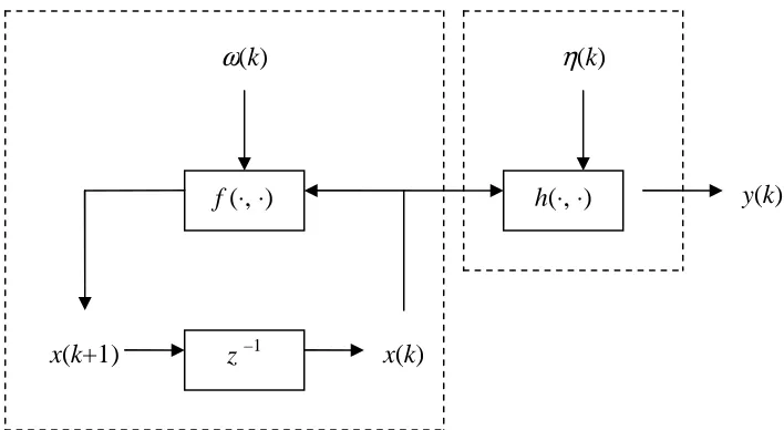
Consider a system model given below.

x(k+1)= f(x(k),k)+ω(k) (1.1) where k denotes the discrete time step, the vector x(k) denotes the current state, and

) 1 (k+

x denotes the one-step ahead future state, f(x(k),k) is a vector-valued continuously differential function, and ω(k) denotes the process noise. It is assumed that ω(k) is the zero-mean white noise sequence, and that f(x(k),k) does not depend on the previous values of x(k−τ),

τ

= 1, …, k. Thus, this process is a Markov process (Bryson, 2002). The vector x(k) is a state vector and the conditional probability density function (PDF) for x(k) , denoted by

)) ( | ) 1 (

(x k x k

p + , is sometimes called the hyperstate of the process. It is characterized by the mean and the covariance (Torsten, 1994) of the process.

Additional, an observation model is given below. ) ( ) ), ( ( )

(k h x k k k

8

where the vector y(k) denotes a set of observables, h(x(k),k) is a vector-valued continuously differentiable function and the vector η(k) denotes the measurement noise. It is assumed that η(k) is a zero-mean measurement white noise sequence.

From (Bryson, 2002), it is also assumed that (a) η(k) and η( j) are independent if k ≠ j, and

(b) x(k), ω(k) and η( j) are statistically independent for all k and j. These assumptions assert that

)) ( | ) 1 ( ( )) ( ), ( | ) 1 (

(x k x k y k p x k x k

p + = + .

[image:29.595.142.496.391.585.2]

The coupling of the system model and the observation model is the state-space model of the stochastic dynamical system. The signal-flow graph representation (Lewis, 1992) of this state-space model is expressed in Figure 1.1.

Figure 1.1 State-space model, where z –1 denotes time-delay unit z –1

f (⋅, ⋅) h(⋅, ⋅)

x(k+1) x(k)

y(k)

9

1.3.3 Optimal Control of Stochastic System

Consider the optimal control of a stochastic system given below.

x(k+1)= f(x(k),u(k),k)+ω(k) (1.3) ) ( ) ), ( ( )

(k h x k k k

y = +η (1.4)

where the vector u(k) is the control variable to be determined such that the following cost functional

∑

− = + = 1 0 )] ), ( ), ( ( ) ), ( ( [ ) ( N k k k u k x L N N x E u

J

ϕ

(1.5)

is minimized, where E denotes the mathematical expectation, J is a scalar expected value,

ϕ

is the terminal cost and L is the cost measure under summation. Note that L is a general time-varying scalar function in terms of the state and control variables at each k for k = 0 to k = N – 1. It is assumed that

ϕ

and L are continuously differentiable functions with respect to their respective arguments.

This is a general class of nonlinear stochastic optimal control problems in discrete-time, where the probability density function (PDF) of the state variables is unknown, but their error covariance can be calculated (Bryson, 2002).

1.4 Motivation and Background of the Study

10

Furthermore, real-world problems are often modelled as nonlinear dynamical systems subject to stochastic disturbances. In this thesis, only the Gaussian white noise is considered. It is known that a complex dynamical system is difficult to be solved analytically. For mathematical tractability, it is assumed that the corresponding functions in the nonlinear system are continuously differentiable functions. As such, the solution, which is in the forms of expectation and filtering, is to be calculated by using appropriate numerical schemes.

By virtue of the efficiency of the model-reality differences approach to the deterministic nonlinear control system, the goal of this thesis is to develop an efficient and effective computational approach based on the principle of model-reality differences to a class of nonlinear discrete-time stochastic optimal control problems. The principle of model-reality differences is not applicable to continuous-time nonlinear stochastic control systems. It is a future research topic.

1.5 Objectives and Scope of the Study

11

Here, we summarize our research objectives as follows.

• To review the existing approaches for solving the nonlinear stochastic optimal control problems.

• To develop an efficient and effective computational approach based on the principle of model-reality differences for a class of nonlinear discrete-time stochastic optimal control problems.

• To apply the optimal state estimate for the nonlinear state estimation.

• To design a feedforward-feedback optimal control law such that the dynamic of discrete-time stochastic system can be stabilized.

• To propose an effective computational methodology for discrete-time stochastic dynamic optimization.

In addition, the scope of our research covers

• Linear and nonlinear stochastic optimal control in discrete-time; • Linear and nonlinear state estimation using Kalman filtering theory;

• Minimum output residual with the concept of the weighted least-square approach;

• Convergence, optimality and stability for the discrete-time stochastic dynamic optimization; and

• Stochastic modelling with the Gaussian white noises.

1.6 Significance of the Study

12

The significance of this study includes

(a) Comprehensive review of literature

Various computational methods are reviewed. Most of the computational schemes are based on approximation. Others are based on the probability density function. This literature review leads us to the study in the thesis.

(b) Algorithm development

A class of integrated optimal control and parameter estimation (IOCPE) algorithms is developed based on the principle of model-reality differences. There are three sub-algorithms listed below.

(i) The ICEES algorithm, which looks for the expectation solution; (ii) The ICEFS algorithm, which computes the filtering solution; and (iii) The ICERS algorithm, which generates the real output solution. They are coded in MATLAB version 7.0 (R14) and implemented in Microsoft Window XP, Pentium M, 496 MB.

(c) Application of optimal state estimate

In the presence of the random disturbances, the best state estimates are (i) the expected state when there is no observation; and (ii) the filtered state when the observation is available. The optimal state estimate generated from Kalman filtering theory is applied instead of using the extended Kalman filter. The online calculation of the filter gain is avoided during the iterative procedure. This will save the computation time of the state estimation.

(d) Design of optimal control law

13

(e) Computational methodology for optimization

The computational methodology integrates the computation of the adjustable parameters and the optimization of the modified model-based optimal control problem interactively in a unified framework. Hence, the model-based optimal control problem is solved instead of solving the original optimal control problem. As a result, the true optimal solution of the original optimal control problem could be obtained in spite of the model-reality differences. This methodology is effective for the discrete-time stochastic optimal control problems.

1.7 Overview of Thesis

In the previous section, comprehensive introductions to the model-reality differences approach and the optimal control of stochastic dynamical systems were given. In particular, the evolution of the model-reality differences approach was reported and the discrete-time nonlinear stochastic optimal control problem was described. The purpose of this thesis is to present new algorithms based on the principle of model-reality differences for solving the discrete-time nonlinear stochastic optimal control problems. The literature review, the development of these algorithms and the theoretical analysis are briefly described below.

In Chapter 2, a brief introduction of the principle of model-reality differences is given. Various types of random processes are described and dynamic estimation, which is carried out from Kalman filtering theory, is discussed. In addition, the relation of smoothing and filtering is revealed. Furthermore, the optimal control of a nonlinear stochastic system is considered, where the stochastic value function and the stochastic Hamiltonian function are presented. For a linear stochastic control system, the dynamic regulator and its optimal control are derived. Finally, some recent results on stochastic control strategies are reviewed.

14

In Chapter 3, the principle of model-reality differences is explained through introducing an expanded optimal control problem. Applying the mean propagation equation to the state dynamic of the stochastic system, the stochastic control system is transformed into a nonlinear deterministic control system. On this basis, the ICEES algorithm with the linear quadratic regulator (LQR) optimal control model, similar to the DISOPE algorithm, is developed. It can then be used to obtain the true expected solution of the original optimal control problem.

In Chapter 4, the observation is considered available. The optimal state estimate is derived from Kalman filtering theory. The off-line computation of the filter gain and the corresponding state error covariance is performed before the iterative procedure begins. The extension of the principle of model-reality differences is carried out such that the ICEFS algorithm is developed. By using the linear quadratic Gaussian (LQG) optimal control model in the algorithm proposed, the true filtering solution of the original optimal control problem is obtained.

In Chapter 5, an improvement on the methodology discussed in Chapter 4 is made. The weighted least-square output residual is introduced and is combined with the cost functional of the model-based optimal control problem. Again, applying the principle of model-reality differences, the corresponding version of the ICERS algorithm is derived. It is important to note that the weighting matrix with the smallest value shall be determined. As such, the true real output solution of the original optimal control problem can be tracked. Eventually, the minimum output residual reduces the noisy level of the problem.

15

CHAPTER 2

LITERATURE REVIEW

2.1 Introduction

The aim of this chapter is to give a detailed overview of the model-reality differences approach and the computational issues of stochastic optimal control problems. On this basis, efficient algorithms are developed based on the principle of model-references for solving nonlinear stochastic optimal control problems in discrete-time.

Firstly, this chapter begins with a discussion on the model-reality differences approach and its application to solve a class of nonlinear deterministic optimal control problems, where the true optimal solution of the nonlinear optimal control problem is obtained without having to solve the original optimal control problem. The resulting algorithm aims to satisfy the necessary optimality conditions, while solving the parameter estimation problem and optimizing the model-based optimal control problem iteratively. In this way, the parameters are iteratively adapted in response to the differences between the real plant and the model used. Then, the optimal solution of the model-based optimal control problem is updated iteratively.

17

function are discussed. For a linear stochastic control system, the control law is derived using the linear quadratic Gaussian technique and the dynamic programming approach. The duality of the estimation and the control is given through the separation principle. In addition, some recent results on stochastic control strategies are reviewed. Finally, some concluding remarks are made and a summary showing the study direction of the thesis is given.

2.2 Nonlinear Optimal Control with Model-Reality Differences

Generally, applying the linear optimal control model to solve a nonlinear optimal control problem is a challenging task. However, if the function of the plant dynamic (also called as reality) is continuously differentiable, then a mathematical model can be formulated from the linearization of the plant dynamic. The solution of the linear optimal control model can be obtained readily. However, solving the linear optimal control problem does not provide the optimal solution to the nonlinear optimal control problem. It is important to fill the gap by reducing the differences between the reality and the model employed.

2.2.1 General Nonlinear Optimal Control Problem

Consider a general optimal control problem, referred to as the real optimal control problem (ROP), given below.

min ( ) ( ( ), ) )

(k Jp u x N N

u =

ϕ

∑

− = + 1 0 ) ), ( ), ( ( N k k k u k x

L (2.1)

subject to ) ), ( ), ( ( ) 1

(k f x k u k k

x + = (2.2)

0 ) 0

( x

x = (2.3)

where x(k)∈ℜn , k =0,L,N, is the real state sequence, u(k)∈ℜm , , 1 , , 0 − = N

18

n m

n

f :ℜ ×ℜ ×ℜ→ℜ represents the real plant (also called reality). J_p∈ℜ is the real cost function, where ℜn ×ℜ→ℜ

:

ϕ

is the terminal cost and

ℜ → ℜ × ℜ ×

ℜn m

L : is the cost under summation. Note that L is a general time-varying scalar function in terms of the state and control variables at each k for k = 0 to k = N – 1. It is assumed that all functions in (2.1) and (2.2) are continuously differentiable with respect to their respective arguments.

The Problem (ROP) is a general deterministic nonlinear optimal control problem. It satisfies the following necessary conditions for optimality (Young, 1969; Pontryagin et al, 1962; Hestenes, 1966; Leitmann, 1981).

) ( ) ( k u k H ∂ ∂ 0 ) 1 ( ) ( ) ), ( ), ( ( ) ( ) ), ( ), ( ( _{+ =}       ∂ ∂ + ∂ ∂

= p k

k u k k u k x f k u k k u k x L T (2.4) ) ( ) ( ) ( k x k H k p ∂ ∂

= ( 1)

) ( ) ), ( ), ( ( ) ( ) ), ( ), ( ( ₊       ∂ ∂ + ∂ ∂

= p k

k x k k u k x f k x k k u k x L T (2.5) ) ), ( ), ( ( ) 1 ( ) ( ) 1

( f x k u k k

k p k H k x = + ∂ ∂ =

+ (2.6)

for k =0,L,N −1,with the boundary conditions

) ( ) ), ( ( ) ( N x N N x N p ∂ ∂

=

ϕ

and x(0)= x₀.

Here, p(N) is the final co-state and x(0) is the initial state, and the function ℜ → ℜ × ℜ × ℜ ×

ℜn m n

H : is the Hamiltonian function defined by

) ), 1 ( ), ( ), ( ( )

(k H x k u k p k k

H = +

=L(x(k),u(k),k)+ p(k+1)T f(x(k),u(k),k) (2.7)

19

Bazaraa et al, 2006; Hull, 2003). For example, the finite difference method and the shooting method are common approaches to solve TPBVP defined by (2.5) and (2.6). The approach proposed in (Teo et al, 1991) solves the problem as an optimization problem. In fact, this approach works for a much general class of problems, where constraints on the state and the control variables are allowed to appear in the problem formulation. The approach proposed in (Hargraves and Paris, 1991) is another approach to solve Problem (ROP) numerically. Others interested approaches are multiparametric quadratic programming (Tøndel, 2003) and Gauss pseudospectral transcription (Benson, 2005).

2.2.2 Linear Model-Based Optimal Control Problem

Because the structure of the real plant is complex, a linear optimal control problem is constructed and is solved instead of solving Problem (ROP). This linear optimal control problem is a linear quadratic regulator (LQR) optimal control model, which is constructed as a simplified model-based optimal control problem (MOP) given below. ) ( ) ( ) ( ) ( ) (

min ₂1

)

( J u x N S N x N N

T m

k

u = +

γ

∑

− = + + + 1 0 2

1_{( ( ) ( ) ( ) ( )) ( )}

N k T T k k Ru k u k Qx k

x γ (2.8)

subject to

x(k+1)=Ax(k)+Bu(k)+α(k) (2.9) 0

) 0

( x

x = (2.10)

where α(k)∈ℜn, k =0,L,N −1, and γ(k)∈ℜ, k =0,L,N, are the adjustable parameters, while A∈ℜn×n is a state transition matrix and B∈ℜn×m is a control coefficient matrix. J_m∈ℜ is the model cost function, where S(N)∈ℜn×n and

n n

20

Notice that the adjusted parameters α(k) and γ(k) are introduced to capture the nonlinear behavior of the reality and they are used to reduced the differences between the reality and the model used. When their values are zero, Problem (MOP) is actually a standard linear quadratic regulator (LQR) optimal control problem. In the literature, this linear optimal control problem is well studied. See, for example, (Slotine and Li, 1991; Speyer, 1986; Lee and Marckus, 1986; Chen, 1984; Kirk, 1970; Walsh, 1975; Bryson and Ho, 1975; Lewis, 1986).

The linear optimal control problem is much easier to be solved. It is because the corresponding TPBVP is a system of linear homogeneous differential equations. Unlike the general nonlinear TPBVP, it can be solved by using the transition matrix method or the backward sweep method (Bryson and Ho, 1975; Lewis, 1986). The transition matrix method is conceptually easy but the difficulty may arise during the computation of the inverse of the transition matrices. The backward sweep method is more popular (Teo et al, 1991) due to the assumption of a linear relationship between the state and the costate for the computational efficiency.

2.2.3 Principle of Model-Reality Differences

The structure of the reality in Problem (ROP) is nonlinear, while the structure of the model used in Problem (MOP) is linear. The methodology which is proposed to reduce the differences between the reality and the model used is known as the principle of model-reality differences. In this principle, Problem (MOP), instead of Problem (ROP), is solved in such a way that the true solution of Problem (ROP) is obtained despite model-reality differences by updating the adjustable parameters iteratively.

21

min ( ) ₂1 ( ) ( ) ( ) ( ) )

(k Je u x N S N x N N

u = +

γ

) ( )) ( ) ( ) ( ) ( ( 1 0 2

1 _{x k Qx k u k Ru k k}

N

k

T

T _{+ +}γ

+

∑

− =

2 ₂1 ₂ 2

1 2

1_{r ||u(k)}−_v(k)|| + _{r ||x(k)}−_z(k)||

+ (2.11)

subject to

x(k+1)= Ax(k)+Bu(k)+α(k) (2.12) 0

) 0

( x

x = (2.13)

) ), ( ( ) ( ) ( ) ( ) ( 2

1_{z N} T_{S N z N} +γ _N =ϕ _{z N N}

(2.14) 1₂(_z(_k)T_Qz(_k)+_v(_k)T_Rv(_k))+γ(_k)=_L(_z(_k),_v(_k),_k)

(2.15) ) ), ( ), ( ( ) ( ) ( )

(k Bv k k f z k v k k

Az + +α = (2.16)

) ( ) (k x k

z = (2.17)

) ( ) (k u k

v = (2.18)

where v(k)∈ℜm , k =0,L,N −1, and z(k)∈ℜn , k =0,L,N, are introduced to separate the control sequence and the state sequence in the optimization problem from the respective signals in the parameter estimation. The terms appearing with

ℜ ∈ 1

22

2.2.4 Optimality Conditions

Now, let us define the Hamiltonian function of Problem (EOP) as follows. ( ) 2( ( ) ( ) ( ) ( )) ( )

1 _{x k Qx k u k Ru k k}

k

He = T + T +γ

2 2 2 1 2 1 2

1_{r ||u(k)}−_v(k)|| + _{r ||x(k)}−_z(k)|| +

+p(k+1)T(Ax(k)+Bu(k)+

α

(k))

−

λ

(k)Tu(k)−

β

(k)Tx(k) (2.19) Then, we append the system (2.12) and the additional constraints (2.14) – (2.18) to the cost function (2.11), in terms of H_e(k), to define the augmented cost function as follows. ) ( ) ( ) ( ) ( )

(_{u 2}1 _{x N S N x N N}

J_e′ = +

γ

+ p(0)Tx(0)−p(N)Tx(N) )) ( ) ( ) ( ) ( ) ), ( ( )(

(_N

ϕ

_{z N N 2}1 _{z N} T_{S N z N}

γ

_N

ξ

− −

+

)) ( ) (

(x N z N

T − Γ +

∑

− = − + 1 0 ) ( ) ( ) ( N k T

e k p k x k

H +

λ

(k)Tv(k) +

β

(k)Tz(k)

)) ( )) ( ) ( ) ( ) ( ( ) ), ( ), ( ( )(

(_{k L z k v k k 2}1 _{z k} T_{Qz k v k} T_{Rv k}

γ

_k

ξ

− + −

+ )) ( ) ( ) ( ) ), ( ), ( ( ( )

(k T f z k v k k Az k Bv k

α

k

µ

− − −

+ (2.20)

where

λ

(k)∈ℜm, k =0,L,N −1,

β

(k)∈ℜn, k =0,L,N −1, Γ∈ℜn, ξ(k)∈ℜ, ,

, ,

0 N

k = _L and n

k)∈ℜ (

µ , k =0,_L,N −1, are the appropriate Lagrange multipliers.

According to the Lagrange multiplier theory, the first-order variation δJe′ of

the augmented cost function J_e′ with respect to all variables shall be zero at a constrained minimum (Bryson and Ho, 1975; Lewis, 1986; Becerra, 1994). That is,

0

e

J

23

(a) Stationary condition 0 ) ( )

( =

∇u k He k :

0 )) ( ) ( ( ) ( ) 1 ( )

(k +B p k+ − k +r1 u k −v k =

Ru T

λ

(2.21)

(b) Co-state equation ) ( )

(k _{( )}H k p =∇_{xk e} :

) ( ) 1 ( ) ( )

(k Qx k A p k k

p = + T + −

β

+r₂(x(k)−z(k)) (2.22)

(c) State equation

) ( )

1

(k _{( 1)}H k

x + =∇_{p k+ e} :

) ( ) ( ) ( ) 1

(k Ax k Bu k k

x + = + +α (2.23)

(d) Boundary conditions ) ( ) ( )

(N S N x N

p = +Γ and x(0)= x0

(e) Parameter estimation equations

0 ) ( ) ( ) ( ) ( ) ), (

(_{z N N} −1_{2 z N} T_{S N z N} −γ _N =

ϕ (2.24a)

0 ) ( )) ( ) ( ) ( ) ( ( ) ), ( ), (

(_{z k v k k} −1_{2 z k Qz k} +_{v k Rv k} − _k =

L T T γ (2.24b)

0 ) ( ) ( ) ( ) ), ( ), (

(z k v k k −Az k −Bv k − k =

f α (2.24c)

(f) Modifier equations

0 ) ( ) ( )

( − −Γ=

∇z Nϕ S N z N (2.25a)

0 ) 1 ( ˆ ) ( )) ( ( ) ( ( )  + =      − ∂ ∂ + − ∇

+ B p k

k v f k Rv L k T k v

λ (2.25b)

)) ( (

)

(k + ∇z(k)L−Qz k

β ˆ( 1) 0

) (  + =     − ∂ ∂

+ A p k

k z

f T

(2.25c) with ξ(k)=1 and µ(k)= pˆ(k+1).

(g) Separation of variables ) ( ) (k u k

24

2.2.5 Relevant Problems from Integration

After satisfying the optimality conditions of Problem (EOP) defined by (2.21) – (2.26), the modified model-based optimal control problem (MMOP) is obtained as follows. ) ( ) ( ) ( ) ( ) (

min ₂1

)

( J u x N S N x N N

T mm

k

u = +

γ

x(N)

T Γ +

∑

− = + + + 1 0 2

1_{( ( ) ( ) ( ) ( )) ( )}

N k T T k k Ru k u k Qx k x γ 2 2 2 1 2 1 2

1_{r ||u(k)}−_v(k)|| + _{r ||x(k)}−_z(k)|| +

−λ(k)Tu(k)−β(k)Tx(k) (2.27) subject to

x(k+1)= Ax(k)+Bu(k)+α(k) (2.28) 0

) 0

( x

x = (2.29)

with the specified α(k) , γ(k), λ(k), β(k), Γ , v(k) and z(k) that are being calculated.

In addition, (2.24) defines the parameter estimation problem. From this problem, the adjustable parameters are determined by

) ), ( ( )

(N ϕ z N N

γ = −1_{2 z}(_N)T_S(_N)_z(_N)

(2.30a) ) ), ( ), ( ( )

(k =L z k v k k

γ −1₂(_z(_k)T_Qz(_k)+_u(_k)T_Ru(_k))

(2.30b) ) ), ( ), ( ( )

(k = f z k v k k

α −Az(k)−Bv(k) (2.30c)

and from the multipliers computation defined by (2.25), the multipliers are calculated from ) ( ) ( )

(N S N z N

z −

∇ =

Γ ϕ (2.31a)

) 1 ( ˆ ) ( )) ( ( ) ( ( )  +      − ∂ ∂ − − ∇ −

= B p k

k v f k Rv L k T k v

λ (2.31b)

)) ( (

)

(k =− ∇z(k)L−Qz k

β ˆ( 1)

) (  +     − ∂ ∂

− A p k

k z

f T