332
Domain Decomposition Method for Solving
Incompressible Fluid Flow and Energy Equations using
Distributed Parallel Computer System
Bukhari bin Manshoor
LecturerFaculty of Mechanical & Manufacturing Engineering University Tun Hussein Onn Malaysia
+607-4537828
[email protected]
ABSTRACT
This paper is concerned with the development of an efficient scheme for solving the finite difference Navier-Stokes and energy equations using distributed parallel computer system. The numerical procedure is based on SIMPLE (Semi Implicit Method for Pressure Link Equations) developed by Spalding. The governing equations are transformed into finite difference forms using the control volume approach. The hybrid scheme which is combination of the central difference and up wind scheme is used in obtaining a profile assumption for parameter variations between the grids points. Parallelization method used on this distributed parallel computer system is Domain Decomposition Method (DDM). The accuracy of the parallelization method is done by comparing with a benchmark solution of a standardized problem related to the two dimensional buoyancy flow in a square enclosure. The results shown that the distributed parallel computer system will reduced an execution time to solve the problem about 70% compared to the serial computer.
Keywords
SIMPLE algorithm, Parallel Algorithm, Domain Decomposition Method, Navier-Stokes Equations.
1. INTRODUCTION
The equations governing the fluid dynamics and energy flow have been know for the most part for more than a century and yet have continued to defy analytical solution. Instead their solutions have largely been obtained by experimental simulations in wind tunnels, water tables and shock tubes [4]. Now with the ability of advanced scientific computer such as distributed parallel computer system, the equations can be solved using the methods of computational fluid dynamic (CFD). Now, it surprising that, fluid dynamics and heat transfer are contributing to and benefiting from current development in finite difference numerical analysis. In recent years, several finite difference schemes have been proposed and develop. Some methods have used the primitive variables, while some have solved the equations in terms of
vorticity and stream function as the dependent variables. The governing equations are often transformed into the non-dimensional form. The advantage is that it is more convenient to work with dimensionless variables. The characteristic parameter such as Reynold number, Prandt number and Rayleigh number can be varied independently. Furthermore, by non-dimensionalising the equations, the flow parameters such as velocity and temperature are normalized so that their values can be adjusted to fall between certain prescribed limits. A number of general purpose computer programs using finite difference methods have been developed. Some of these programs using serial computer have relied on works of the Argonne National Laboratory Group, Illinious, USA [5] and methods based on the works at Imperial College, London [8].
This paper deals with a development of an efficient scheme for solving the finite difference Navier-Stokes and energy equations using distributed parallel computer system. The numerical procedure is based on SIMPLE (Semi Implicit Method for Pressure Link Equations) developed by Spalding [2]. As we know, the analysis of an incompressible flow become more complicated and need a high performance computer to solve the problem. One of the problem during to solve the complicated problem on incompressible flow is time constraint. More complicated of the problem means more time should be spend to solve the problem.
333
2. NUMERICAL ANALYSIS
2.1 Governing equations
Two-dimensional incompressible laminar constant-density flow [7] and energy equation is governed by set of partial differential equations. The continuity, momentum and energy equations in their primitive form are shown in equation (1-4) where the equation for conservation of mass is given by:
=0 ∂ ∂ + ∂ ∂ y v x
u (1)
The conservation of momentum in x and y directions are governed by the u-momentum equation expressed as:
( ) ( )
(
)
(
)
x k L H y u H L Ra x p L H x u L H Ra y uv x uu t t ∂ ∂ − + ∂ ∂ + ∂ ∂ − + ∂ ∂ = ∂ ∂ + ∂ ∂ − − 3 2 1 Pr 1 Pr 2 2 4 / 1 2 2 4 / 1ν
ν
(2)as well as the v-momentum equation:
( ) ( )
(
)
(
)
Ra
T
L
H
y
k
H
L
y
v
H
L
Ra
y
p
H
L
x
v
L
H
Ra
y
vv
x
uv
t t 2 / 1 2 2 4 / 1 2 2 4 / 1Pr
3
2
1
Pr
1
Pr
+
∂
∂
−
+
∂
∂
+
∂
∂
−
+
∂
∂
=
∂
∂
+
∂
∂
− −ν
ν
(3)The conservation of energy will express as:
( ) ( )
+ ∂ ∂ + ∂ ∂ = ∂ ∂ + ∂ ∂ − − t T T T y T H L Ra x T L H Ra y vT x uTν
σ
ν
σ
Pr 1 Pr 1 2 2 4 / 1 2 2 4 / 1 (4)In the above equations, u and v are the x and y components of the velocity, p is the pressure, ρ and ν are the density and viscosity respectively.
2.2 Finite Difference Equations
In the development of the control volume approach, the governing partial differential equations are first transformed into divergence force. Let the dependent variables (u, v, and T) are denoted by Ø, the general differential equation can be written as:
div
( )
ρuφ =div(
Γgradφ)
+Swhere Γ is the diffusion coefficient, or:
div
(
ρ
u
φ
−
Γ
grad
φ
)
=
S
When the above finite difference scheme is applied to each momentum equation, the final difference equations can be written as: =
∑
+ +(
−)
i E P u nb nb PPu P P y
L H b u a u a (5) =
∑
+ +(
−)
j N P v nb nb PPv P P x
H L b v a v a (6)
The summations are over the four neighboring velocities where nb in above equations denotes neighbors.
2.3 Correction Equation
In the SIMPLE method, the true pressure field, P, which will produce the true velocity fields satisfying the continuity equation is given as:
'
P P
P= ∗+ (7)
where P’ is the pressure correction. Similarly, the true velocity fields are given by:
' ' v v v u u u + = + = ∗ ∗ (8)
where u’ and v’ are the velocity corrections. Expressions for these velocity corrections can be obtained from the momentum equations and they are of the forms:
(
)
E P Pu
i P P
a y L H
u'= ' − ' (9)
(
)
E P Pv j P P a x H Lv'= ' − ' (10)
The true velocity fields are then obtained by adding the intermediate velocity fields to the velocity corrections. For the control volume shown the true velocity fields can be written as:
(
)
E P pe i pp P P
a y L H u
u = ∗+ ' − ' (11)
(
)
N P pn j pp P P
a x
H L v
v = ∗+ ' − ' (12)
(
)
P W pw i ww P P
a y L H u
u = ∗+ ' − ' (13)
(
)
P S ps j ss P P
a x
H L v
v = ∗+ ' − ' (14)
We now turn to the task of deriving a difference equation for the pressure correction using the continuity equation. The integrated continuity equation is given by:
F
e−
F
w−
F
n−
F
s=
0
or:− + − =0
j s j p i w i
py u y v x vx
334 Substitute the expressions given in equations (11) to (14) for all the velocity components into equation (15), we have:
a P a P a P a P a P b
PS S N N W W E P
P ' = E ' + ' + ' + ' + (16)
where:
pe i E
a y L H a
2 =
pw i W
a y L H a
2 =
pn j N
a x
H L a
2
=
ps j S
a x
H L a
2
=
S N W E
P a a a a
a = + + +
j p j s i p i
w y u y v x v x
u
b= ∗ − ∗ + ∗ + ∗
2.4 Solution of the Differential Equation
When all the governing equations are transformed into finite difference form, we have a set of algebraic equations which can be solved by any suitable method. For the present calculations, we have employed a line by line iteration method on distributed parallel computer system. Parallelization method used known as Domain Decomposition Method (DDM). Using this method, a grid line is chosen and the values of Ø for the nodes along the chosen line are assumed to be unknowns. However, the values of
Ø for the nodes along the neighboring lines are assumed to be known and these values are taken from previous iteration. The equations for the grid points along the chosen line are then solved using tridiagonal matrix algorithm (TDMA).
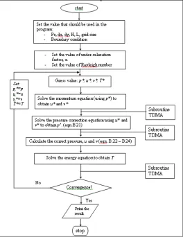
2.5 Solution Procedure of the SIMPLE Algorithm
The SIMPLE method proceeds by a cyclic series of guess and correct operations. The important operations are described in the following steps below. The flow chart of the algorithm was showed in Figure 1.
i. Guess the pressure field, p*.
ii. Solve the momentum equation to obtain u* and v*. iii. Solve the pressure correction equation to obtain p’. iv. Calculate p form equation “
p
=
p
* p
+
'
” by adding p’to p*.
v. Calculate u and v from their starred values using velocity correction equation.
vi. Solve the discretization equation for other ø’s (for this case, we solve the energy equation to obtain temperature T) vii. Treat the corrected pressure p as new guessed p*, return to
[image:3.612.313.577.72.414.2]step 2 and repeat the whole procedure until a converged solution is obtained.
Figure 1. Flow chart of SIMPLE algorithm.
3. PARALLEL IMPLEMENTATION
A parallel implementation can provide a further reduction in computing time. Parallel implementation also makes solution possible to problems that would require too much memory to solve on a single processor. During to solve this problem, the parallel implementation is based on message passing (distributed memory systems) using the PVM software. Portability is ensured because PVM is available on many types of parallel computers. The implementation uses a layer of subroutines on top of PVM, symbolically denoted by;
start: start entire parallel application
stop: stop parallel application
send: send a message
receive: receive a message
3.1 Communication Process
335
find out if I am MASTER or SLAVES
if I am MASTER initialize array
send each SLAVES starting info and subarray
do until all SLAVES converge
gather from all SLAVES convergence data broadcast to all SLAVES convergence signal end do
receive results from each SLAVE
else if I am SLAVE
receive from MASTER starting info and subarray
do until solution converged update time
send neighbors my border info receive from neighbors their b order info
update my portion of solution array
determine if my solution has converged send MASTER convergence data receive from MASTER convergence signal end do
send MASTER results endif
Figure 2. Pseudo code solution.
3.2 Communication
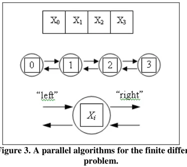
[image:4.612.318.562.362.579.2]Basically this finite difference problem is same with the solution of the problem in this project. From top to bottom of the Figure 3; the one-dimensional vector X, where N=4; the task structure, showing the 4 tasks, each encapsulating a single data value and connected to left and right neighbors via channels; and the structure of a single task, showing its two inports and outports.
Figure 3. A parallel algorithms for the finite difference problem.
We first consider a one-dimensional finite difference problem, in which we have a vector X( )0of size N and must computeX( )T , where;
( ) ( ) ( ) ( )
4 2 :
0 , 1
0 1 1
t i t i t i t i
X X X X T t N
i< − ≤ < + = + + +
<
That is, we must repeatedly update each element of X, with no element being updated in step t+1 until its neighbors have been updated in step t. A parallel algorithm for this problem creates N tasks, one for each point in X. The ith task is given the value
( )0
X and is responsible for computing, in T steps, the values ( ) ( ) ( )T
i i
i X X
X 1, 2,..., .
Hence, at step t, it must obtain the values ( )t i
X−1 and ( )t i
X+1 from
tasks i-1 and i+1. We specify this data transfer by defining channels that link each task with “left” and “right” neighbors, as shown in Figure 3, and requiring that at step t, each task i other than task 0 and task N-1
i. sends its data ( )T i
X on its left and right outports,
ii. receives ( )t i X−1 and
( )t i
X+1 from its left and right inports,
and
iii. use these values to compute ( )t+1
i
X .
Notice that the N tasks can execute independently, with the only constraint on execution order being the synchronization enforced by the receive operations. This synchronization ensures that no data value is updated at step t+1 until the data values in neighboring tasks have been updated at step t. Hence, execution is deterministic.
C broadcast data to slaves
call pvmfinitsend (PVMDEFAULT, info) call pvmfpack (INTEGER4, nproc, 1, 1, info) call pvmfpack (INTEGER4, tids, nproc, 1, info) call pvmfpack (INTEGER4, n, 1, 1, info) call pvmfpack (REAL8, data, n, 1, info) msgtype = 1
call pvmfmcast (nproc, tids, msgtype, info)
C wait for results from slaves
msgtype = 2 do 30 i = 1,nproc
call pvmfrecv (-1, msgtype, info)
call pvmfunpack (INTEGER4, who, 1, 1, info) call pvmfunpack (REAL8, result(who+1), 1, 1, info) if (who.eq.0)
then
write (*,1000) result(who+1), who, (nroc-1) else
write (*,1000) result(who+1), who, 2*(who-1) 30 continue
[image:4.612.73.260.462.629.2]336
C receive data from master
msgtype = 1
call pvmfrecv (mtid, msgtype, info)
call pvmfunpack (INTEGER4, nproc, 1, 1, info) call pvmfunpack (INTEGER4, tids, nproc, 1, info) call pvmfunpack (INTEGER4, n, 1, 1, info) call pvmfunpack (REAL8, data, n, 1, info)
C determine which slave I'm (0...nproc-1)
do 5 i = 0,nproc if (tids(i).eq.mytid) me = i 5 continue
C do calculation with the data
result = work (me, n, data, tids, nproc)
C send the result to the master
call pvmfinitsend (PVMDEFAULT, info) call pvmfpack (INTEGER4, me, 1, 1, info) call pvmfpack (REAL8, result, 1, 1, info) msgtype = 2
[image:5.612.50.303.70.323.2]call pvmfsend (mtid, msgtype, info)
[image:5.612.313.578.94.195.2]Figure 5. Algorithm slaves to receive and send data from and to master.
Figure 4 and 5 above showed the algorithms for the sending and receiving data from master and slaves.
4. DISCUSSION
4.1 Validation of the Results
Table 1 to 3 compared the results from the present simulation with the literature results obtained by de Vahl Davis [2]. The results of de Vahl Davis are the standard against which all other codes have been evaluated. Maximum horizontal velocity on the vertical midplane of the cavity, Umax, maximum vertical velocity on the
horizontal midplane of the cavity, Vmax, and an average of Nusselt
number was compared at Rayleigh numbers of 103, 104, 105 and 106. The comparison was done between the benchmark results obtained by de Vahl Davis which in serial processor and the present study that is simulation using serial processor and parallel processor or parallel computer.
From the tables, it showed that all these results are in excellent agreement with the benchmark results of de Vahl Davis. Percentage error for the three methods of solution is below than 3% compare with benchmark result. Besides that, the result that was showed in the forms of contour maps of non-dimensional temperature and velocities also was compared with the results that obtained by de Vahl Davis.
Table 1. Comparison of the numerical result of present study for Umax
Ra 103 104 105 106
G. de Vahl Davis 3.649 16.193 34.620 64.593
Present study:
i) Serial processor 3.652 16.163 34.871 65.812
% error 0.082 % 0.185 % 0.725 % 1.880 %
ii)Parallel processor 3.592 16.376 34.852 65.847
[image:5.612.312.586.234.331.2]% error 1.560 % 1.131 % 0.670 % 1.941 %
Table 2. Comparison of the numerical result of present study for Vmax
Ra 103 104 105 106
G. de Vahl Davis 3.697 19.167 68.590 216.360
Present study:
i) Serial processing 3.704 19.675 69.482 220.641
% error 0.189 % 2.650 % 1.300 % 1.978 %
ii)Parallel processing 3.715 19.642 69.680 221.282
% error 0.487 % 2.478 % 1.589 % 2.275 %
Table 3. Comparison of the numerical result of present study for
____
Nu
Ra 103 104 105 106
G. de Vahl Davis 1.118 2.243 4.519 8.800
Present study:
i) Serial processing 1.120 2.282 4.583 8.983
% error 0.23 % 1.74 % 1.42 % 2.08 %
ii)Parallel processing 1.123 2.272 4.594 9.008
% error 0.47 % 1.31 % 1.67 % 2.36 %
4.2 Parallel Computing Results
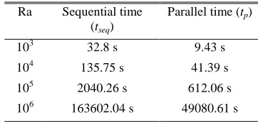
[image:5.612.312.573.358.453.2]In order to achieve the objective of this project, parallel execution time was studied to determine the performance of the parallel computations. Two methods of solution there are serial computation and parallel computation were used during to obtain the results of the simulation. Table 4 showed the results for both methods of computational solution in term of execution time. Table 5 was showed the tabulated results of computational time and communication time for parallel with domain decomposition method.
Table 4. Execution time for three computational solutions
Ra Sequential time (tseq)
Parallel time (tp)
103 32.8 s 9.43 s
104 135.75 s 41.39 s
105 2040.26 s 612.06 s
[image:5.612.345.526.601.687.2]337 Table 5. Computational and communication time for parallel
computation
Ra tcomp tcomm tp
103 8.41 s 1.02 s 9.43 s
104 34.62 s 6.78 s 41.39 s
105 522.82 s 89.24 s 612.06 s 106 41923.02 s 7157.60 s 49080.61 s
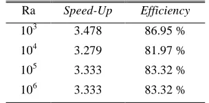
[image:6.612.75.270.95.171.2]Other parameter that was used to measure a performance of parallel computations is up and efficiency. From the speed-up, we know that how fast the parallel computer solves the problem under consideration. It is sometimes useful to know how long processors are being used on the computation, which can be found from the efficiency. Table 6 below was showed result for speed-up and efficiency for parallel methods. Figure 6, 7 and 8 showed graphically an execution time, speed-up and efficiency against number of processors for Ra=103 respectively.
Table 6. Results for speed-up and efficiency
Ra Speed-Up Efficiency
103 3.478 86.95 %
104 3.279 81.97 %
105 3.333 83.32 %
106 3.333 83.32 %
4.3 Discussions
From the results that were obtained, we can see that execution time for parallel computation was decrease compare with sequential computation. By using sequential computation, total execution time that we need to complete our simulation at Rayleigh number 106 is 163602.04 seconds or 2726.7 minutes or 45.45 hours. For parallel computation, we were reduced an execution time for the simulation at Rayleigh number 106 to 49080.61 seconds or 818.01 minutes or 13.63 hours. Compare for both methods of simulations, we got the parallel computation with domain decomposition method is more successful for solve this problem with reducing about 70% of execution time.
From the Figure 6 to 8, we can see an effect of number of processors in parallelization to the execution time, speed-up and efficiency. As we can see, the execution time will decrease with increasing of the number of processors. For the speed-up, it will increase with the increasing of the number of processors. However, the efficiency of a simulation was decrease with an increasing of the number of processors.
0 5 10 15 20 25 30 35
0 1 2 3 4 5
No. of Processors
E
x
e
c
u
ti
o
n
t
im
e
(
s
[image:6.612.320.567.254.398.2])
Figure 6. Execution time against no. of processors for Ra = 103
0 0.5 1 1.5 2 2.5 3 3.5 4
0 0.5 1 1.5 2 2.5 3 3.5 4 4.5
No. of Processors
S
p
e
e
d
-u
p
Figure 7. Speed-Up against no. of processors for Ra = 103
0.86 0.88 0.9 0.92 0.94 0.96 0.98 1 1.02
0 0.5 1 1.5 2 2.5 3 3.5 4 4.5
No. of Processors
E
ff
ic
ie
n
c
y
Figure 8. Efficiency against no. of processors for Ra = 103
5. CONCLUSION
[image:6.612.97.249.299.374.2] [image:6.612.319.567.433.578.2]338 Parallelization using distributed parallel computer system with domain decomposition method can reduce an exection time to solve the problem about 70% by using 4 processors. Therefore it has proved that clustering personal computers together can provide adequate computing power for large engineering problems.
6. ACKNOWLEDGMENTS
Thanks to Faculty of Science, UTM for allowing us to using their Parallel Computer Lab and also to each and everyone who have in any way contributed to this project.
7. REFERENCES
[1] A. W. Date (1985). “Numerical Prediction of Natural Convection Heat Transfer in Horizontal Annulus”. Int. J. Heat Mass Transfer.
[2] Davis G. de Vahl (1983). “Natural convection of air in a square cavity: a benchmark numerical solution”. Int. Journal Numerical Mech. Fluid (3): 249-264.
[3] D. B. Spalding (1972). “A Novel Finite Difference Formulation for Differential Expressions Involving Both First and Second Derivatives.” Int. J. Num. Methods Eng. (3): 551-559.
[4] A. Hayati (1990). “Convective Heat Transfer in Building Energy Analysis”, M. Eng Thesis, Faculty of Mech. Engineering, UTM.
[5] S. P. Vanka, G. K. Leaf (1983). “Fully-Coupled Solution of Pressure-Linked Fluid Flow Equations” Argonne National Laboratory, Argonne, Illinois.
[6] H. K. Versteeg and W. Malalasekera. (1995). “An Introduction to Computational Fluid Dynamics.” Pearson, Prentice Hall.
[7] M. C. Melaaen (1993). “Nonstaggered Calculation of Laminar and Turbulent Flows using Nonorthogonal Coordinates.” Int. J. Num. Heat Transfer: 375-392.
[8] S. V. Patankar (1980). “Numerical Heat Transfer and Fluid Flow.” McGraw-Hill Inc, New York.
[9] S. V. Patankar and D. B. Spalding (1972). “A Calculation Procedure for Heat, Mass and Momentum Transfer in 3-Dimensional Parabolic Flows.” Int. J. Heat Mass Trasfer.
[10] Dongarra, J. & Eijkhout, U. (2000). “Numerical linear algebra algorithms and software.” Journal of Computational and Applied mathematics. 123 (2):489-514.