Progress in Geo Electrical Methods for Hydrogeological Mapping?

Progress in Geo-Electrical Methods for

Hydrogeological Mapping?

Niels Schrøder

Department of Environmental, Social and Spatial Change - ENSPAC Roskilde University *Corresponding Author: [email protected]

Copyright © 2014 Horizon Research Publishing All rights reserved.

Abstract

methods were primarily used for groundwater exploration and the application of the methods were normally followed by a borehole, and a moment of truth. In this process the use of DC (direct current) soundings have been developed to a high grade of excellence. In the last 25 years the geo-electrical methods are more used in connection with groundwater protection and planning, and new methods, as transient electromagnetic (TEM) soundings, have been developed that provide more measurements per hour. In Denmark this change is very explicit, and a paper has – compared results of TEM based mapping with results from wells in a test area north of Aarhus – and stated that: “it is time to do away with the old way of using geophysics”.The present paper tests this statement and concludes that critical boreholes have been overlooked in the analysis. The test area was earlier mapped by DC-soundings, so it is possible to test the methods against each other. It is concluded that well performed DC-soundings with a Schlumberger configuration still provide the best base for hydrogeological mapping.

Keywords

Exploration, Groundwater Protection, Denmark

1. Introduction

In most of the 20th _{century DC (direct current) resistivity}

soundings have been the most used method for hydrogeological mapping. The development of DC soundings for groundwater exploration was helped significantly by the many tests of the predictability of the method - as geo-electrical surveys were normally followed by a drill hole, and a moment of truth. The questions the geophysicist were asked were simple: “Is an aquifer present here and how deep must be drilled?”

However most of the hydrogeological mapping performed in the last 25 years has been for groundwater protection and planning and not for groundwater exploration.

For this type of mapping it has been suggested that other techniques, such as computer-aided interpretation of a dense

net of transient electro-magnetic (TEM) soundings and continuous profiling (tomography) are better suited than the classical methods. These new methods often result in maps and profiles containing innumerabledetails in various colors - apparently of the subsurface geology. Many of the details are however artifacts derived from automatic interpretation of “noise” and do not represent information of the subsurface. The predictability of the methods is very seldom tested by boreholes.

From Denmark a review of hydrogeological mapping by continuous profiling andTEM soundings is used as a base for establishing groundwater protection zones is reported by Thomsen et al. [1].The review concludes, based on results from a test area, that “dense mapping with newly developed geophysical measurement methods -- accords geophysics a highly central role in the forthcoming hydrogeological mapping” and that “surface mapping with the new geophysical methods, combined with better interpretation programmes, has shown that it is time to do away with the old way of using geophysics”.

As this conclusion apparently is based quantitatively by a lot of borehole data, it is increasingly being cited by other authors who advocate the new methods for planning purposes.

The opinion that computer assisted interpretation of a dense net of profiles and soundings could give sufficient information on the subsurface is captivating and planners could be tempted to believe this, - but is it true?

The present paper will investigate this question by reviewing the classical works on the accuracy of the interpretations depending on the accuracy of the measurements, and will test the results of the new methods against the results obtained by the classical Schlumberger soundings measured in the test area.

2. Background

thinking, he constructed the equipment and made the first experiments in Normandy [2]. Many attempts had been carried out by earlier researchers, who had been content to measure the resistance of the earth to a current flowing between two electrodes; a resistance that in practice depends only on the material immediately adjacent to the electrodes.

The first use of the 4 electrodes (two current and two potential electrodes) DC-method was developed for mineral prospecting. However, after 1925, when the first calculations of model-curves for a horizontal stratified earth were performed, the vertical sounding could be interpreted successfully, and the application in hydrogeological mapping started to grow.

3. Development in Measuring

Technology

The most used configurations for vertical soundings have been the Schlumberger configuration (with fixed the potential electrodes) and the Wenner configuration (with continuous increase in the distance between the potential electrodes). Until the 1960th _{the Wenner configuration was}

most in use, as increase in the distance between the potential electrodes allowed the measurements to be performed even with primitive voltmeters. However, as the potential electrodes in the Wenner configuration are moved after each measurement, the measured results are significantly influenced by inhomogeneity in the top soil, so the accuracy in interpretation is low.

As the electronic voltmeters in the 1960th _{became accurate}

and cheap it was then possible to perform Schlumberger configuration soundings with low noise non-polarizable potential electrodes, where the potential electrodes could be fixed with distance “a” at 1 and 10 meters allowing measurements with distance “L” between current electrodes of up to 1 km. The sounding curves then consisted of only two segments representing the 2 distances between the potential electrodes. Already in 1954 Deppermannn [3] investigated the problem in detail and concluded that the offset due to surface inhomogeneity can be substantial - often more than 10 % - and should be corrected by parallel displacement of the segments before interpretation – a correction that cannot be made using the Wenner configuration or continuous profiling (tomography) methods.

4. Development in Interpretation

Methods

Interpretation of the measured sounding curve is traditionally done by comparing it with computed model-curves for horizontal layers. Stefanesco published (1930) in cooperation with C and M Schlumberger methods for calculating model-curves [4], and since Companie Générale de Géophysique in1955 published their atlas, 3-layer curves [5] have been available for everybody. Later,

5-layer curves were published [6], allowing the more tricky problems with double aquifers to be solved.

However Maillet in1947 showed [7], that even if in theory a precise sounding curve over plan-parallel layers would have only one solution, the inhomogeneity in the earth made a determination of points at the curve with an error below 2% impossible and his principles of equivalence and suppression should be used in the interpretation. These principles made it mandatory for a useful interpretation that geological information and information from neighboring soundings was used in order to minimize the ambiguity.

Calculating model-curves were for many years very time consuming. However in 1971 Gosh [8] made it possible to calculate model-curves and do “automatic” interpretation of soundings in seconds (see fig.5). This was however a mixed blessing, as the principles of equivalence and suppression still are valid and the easy possibility to get an “exact” match made it tempting to deliver a mathematical correct interpretation. The danger is that the automatic interpretation would not take into account geological knowledge as applied in the manual interpretation, and the result, though mathematically correct, could in fact be very wrong.

The hydrogeological mapping, performed in the last 25 years has however mostly been for groundwater protection and planning. For these tasks it has been suggested that computer assisted interpretation and techniques such as continuous profiling and transient electro-magnetic (TEM) soundings are better suited, as more data can be measured, and as computer generated maps legitimate planning decisions better than maps using “subjective” geological models. Thomsen et al. [1] have given a review of hydrogeological mapping as a basis for groundwater protection zones in Denmark, using the area north of the city of Aarhus as a test area for the methods. As this area has been surveyed by DC resistivity soundings 30 years earlier [9], it provides a good case to compare the results from the “old” and “new” geophysical methods.

16. Problems in Continuous Profiling

Thomsen et al. [1] state that ”By carrying out measurements with pulled-array, continuous electrical profiling, it has been possible to map contiguous variations within the upper approximately 30 m of the subsurface which would not be possible to map on the basis of borehole data alone”. Measurements with pulled-array continuous electrical profiling are not solving the basic inaccuracy problem of moving potential electrodes over inhomogeneous topsoil, well known from Wenner soundings [3].

However if pulled-array continuous electrical profiling is made in lakes, rivers or shallow seas the “surface layer” is so homogeneous that a measuring precision well below 1% can be obtained if electrochemical stable electrodes are used, and an useful interpretation can be done [10]. As an example resistivity measurement from Roskilde Fjord has been used to map freshwater springs in the fjord indicating where groundwater could be exploited without unwanted side-effects on the base-flow and ecology of streams on land [11].

17. Direct current (DC) Soundings

Versus Transient Electromagnetic

(TEM) Soundings

Aquifers in Denmark often occur in buried valleys eroded into the pre-Quaternary substratum. The buried valleys are typically around 100m deep and often only as much as 1 km wide.

Fig.2 shows two maps by Thomsen et al. representing the test area. Map A shows the pre-Quaternary substratum determined solely from borehole data, and map C showing the pre-Quaternary substratum determined as a results of the transient electromagnetic sounding (TEM) survey in the test area. On this base they claim that the TEM measurements “enable the bed of the buried valleys to be determined“ and “that the new structures identified have now been verified by boreholes”.

Map A shows the pre-Quaternary surface - in the test area - based only on data from boreholes. Map C shows the pre-Quaternary surface, based on transient

electro-magnetic soundings (TEM). On this base Thomsen et al. state that the TEM measurements “enable the bed of the buried valleys to be determined”.

The most dominant example of “new structures identified“ is the buried Ristrup Valley (marked by a red X). However this valley was found by DC-soundings and verified by a borehole already in 1972 (fig.5). The red X in map A and C marks the position of the omitted borehole.

Figure 3. As in fig.2, map C shows the pre-Quaternary surface, based on transient electro-magnetic soundings (TEM). However the same area was earlier

mapped by DC-soundings. As seen in map B from [9] the buried valleys were found in this survey. In maps B and C the test area is marked with a black

square. The red line in map B represents the profile shown in fig.6. Grey color in map C represents suburbs where TEM is affected by noise.

Figure 4. Above is shown the density of data in the test area. Density of boreholes ~3/km2_{. Density of DC-soundings ~1.3km}2_{. Density of TEM ~19/km}2_. Map A and C from [1]. Grey color represents suburbs where TEM is affected by noise.

Based on the DC-soundings the Ristrup Valley was already in the 1970th _{named, by two successive managing directors of}

Aarhus Water Supply [12], as one of the most promising sites for a new groundwater well field for Aarhus. However due to stagnation in water demand the Ristrup well field was not established until 2006.

Due to the fact that DC- soundings from the test area are available, it is possible to test the methods against each other. As seen in fig.3 the buried valleys were found by the DC-soundings. So the real test of the validity of the TEM survey is that it roughly shows the same valleys as were found earlier by DC-soundings.

Comparing the results by Thomsen et al. with the results of the DC-survey it should be stated, that the less dense DC-mapping (fig.4) with more accurate methods gives better hydrogeological maps, and the screen print (fig.5) shows that interactive computer/graphic-display-terminal system for interpretation of resistivity soundings based on the methods developed by Gosh [8], was already developed at the time of the “old” survey.

A low resistivity substratum (in casu the Tertiary clays) gives a good signal with TEM, so there is here not much difference between the TEM and the DC maps of the pre-Quaternary substratum.

Figure 5. Screen print of the interactive computer/graphic-display-terminal system for interpretation of resistivity soundings, developed for the 1974 survey (fig.1.14 in [9]). The figure shows that an automatic and semi-automatic program, that allows inclusion of geological knowledge in the interpretation,

was already developed at that time. The sounding shown is the one that found the sand-aquifer at Ristrup. The red X in fig.2 and 3 marks the position of the

sounding – and borehole.

The sand-aquifer below a till layer is clearly seen in the sounding, and was verified by a borehole showing the base of the sand-aquifer in -96 meter = -52 meter below sea-level.

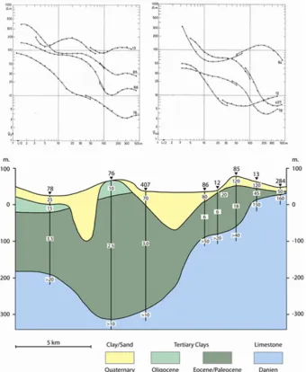
Furthermore the DC-soundings also mapped the limestone aquifer (not mapped by TEM) below the Tertiary clays, as it is seen from the sounding curves in fig.6. The DC-soundings measured outside the deep valleys, allow the true resistivity of the Tertiary deposits to be determined, and the soundings can give very reliable indications, on as well the stratigraphy of the Tertiary clays, as the underlying limestone aquifer.

Figure 6. Schematic profile that shows the tertiary strata in the test area, based on DC-soundings measured outside the buried valleys. The profile is located along the red line in map B (fig.3). Above the profile is shown the DC-soundings on which the interpretation is based. It is seen that the DC-soundings gives very reliable indication on as well top of the tertiary clays as the top of the underlying limestone aquifer. The numbers in the profile indicates the interpreted

18. Conclusions

The aim of the geophysical survey around Aarhus by Thomsen et al. (2004) was to develop new planning tools. The authors conclude that this aim was reached as the survey “demonstrates why dense mapping with newly developed geophysical measurement methods -- accords geophysics a highly central role in the forthcoming hydrogeological mapping”. However their conclusion, that “surface mapping with the new geophysical methods, combined with better interpretation programs, have shown that it is time to do away with the old way of using geophysics” - is not valid. The advances in computer assisted mapping may deliver more colorful and impressive documentation for the planners/politicians, but as the test of quality that boreholes gave to geo-electrical exploration, is seldom applied when geo-electrics are used for planning purpose, it is very important not to oversell the new methods.

The aim to develop a tool for an automatic interpretation of a dense net of geo-electrical data is interesting and has been pursued for many years. However interpretation of geo-electrics is problematic due to noise and the derived ambiguity; and both transient electromagnetic (TEM) soundings as well as pulled-array continuous electrical profiling are very exposed to noise. This is in contrast to classical Schlumberger DC-soundings, where the “old” geophysicist did not leave a sounding site before a smooth (low noise) curve was measured.

The “noisier” the measurements the more important it is to remember the principles of equivalence and suppression in the interpretation, and useful interpretations can only be reached if geological information and information from neighboring soundings is used in order to minimize the ambiguity. This can explain why the results of the new survey in the test area, with ten times more soundings/km2_, thousands of extra measurements with pulled-array continuous electrical profiling, and 30 years of extra knowhow still does not improve upon the old way of using geophysics in the chosen test area.

REFERENCES

[1] Thomsen R, Søndergaard V, Sørensen K (2004):

Hydrogeological mapping as a basis for establishing site-specific groundwater protection zones in Denmark. Hydrogeology Journal.vol.12. nr.5. Springer-Verlag 2004 [2] Kunetz G (1966): Principles of Direct Current Resistivity

Prospecting. Borntraeger, Berlin.

[3] Deppermann K(1954): Die Abhängigkeit des

scheinbaren Widerstandes vom Sonden-abstand bei der Vierpunkt-Methode. Geophysical Prospecting II, p. 62- 73. [4] Stefanesco S (1930) En collaboration avec C. et M.

Schlumberger.: Sur la distributation électrique potentielle autour d’une prise de terre ponctuelle dans un terrain á couches horizontales, homogénes et isotropes. Journal de Physique et le Radium, Série VII, Tome 1.

[5] Compagnie Generale de Geophysique, (I955): Abaques de sondage electrique. Geophysical Prospecting III, suppl. No. 3.

[6] Flathe H (1963): Five-layer master curves for the hydrogeological interpretation of geo- electrical resistivity measurements above a two-storey aquifer. Geophysical Prospecting, XI. 4: 471-508.

[7] Maillet R (1947): The fundamental equations of electrical prospecting. Geophysics 12: 529-556.

[8] Gosh D P (1971): Inverse filter coefficients for the computation of apparent resistivity standard curves, Geophysical Prospecting. Vol. XIX,No.4.

[9] Schrøder N (1974) De geofysisk-geologiske undersøgelser af området nord for Århus. (Geophysical- geological investigations in the area north of Aarhus). In: Frederiksen E, Hastrup H F, Saxov S (eds), Undersøgelser af Århusegnens undergrund. Laboratoriet for Geofysik, Århus Universitet, pp. 11–55. Main hydrogeological mapping results of the above report - in English is in: The hydrogeology of the Trige-Hinnerup area, planning and protection of its groundwater resources. Proceedings . Nordisk Hydrologisk Konference, Aalborg 1974

[10] Schrøder N (1992): Resistivity at Sea. In. R.A.Geyer (edit.), CRC Handbook of Geophysical Exploration at Sea. CRC Press, pp.323-339.

[11] Schrøder N, Højlund Pedersen L, Juel Bitsch R. (2004) 10,000 years of climate change and human impact on the environment in the area surrounding Lejre. The Journal of Transdiciplinary Environmental Studies vol.3 no.1, 2004. [12] Frederiksen E, Hastrup H F, Saxov S (1974): Undersøgelser