Galois and Class Field Theory for Quantum
Chemists
Ichio Kikuchi
1, Akihito Kikuchi
1∗1Internationales Forschungszentrum f¨ur Quantentechnik
June 30, 2020
Abstract
Quantum mechanics could be studied through polynomial algebra, as has been demonstrated by a work (“An approach to first-principles electronic structure calculation by symbolic-numeric computation” by A. Kikuchi). We carry forward the algebraic method of quantum mechanics through al-gebraic number theory; the basic equations are represented by the multi-variate polynomial ideals; the symbolic computations process the ideal and disentangle the eigenstates as the algebraic variety; upon which one can build the Galois extension of the number field, in analogy with the univari-ate polynomial case, to investigunivari-ate the hierarchy of solutions; the Galois extension is accompanied with the group operations, which permute the eigenstates from one to another, and furnish the quantum system with a non-apparent symmetry. Besides, this sort of algebraic quantum mechanics is an embodiment of the class field theory; some of the important conse-quences of the latter emerge in quantum mechanics. We shall demonstrate these points through simple models; we will see the use of computational algebra facilitates such sort of analysis, which might often be complicated if we try to solve them manually.
Keywords— quantum mechanics; algebraic geometry; algebraic number theory; commutative algebra; Gr¨onber basis; primary ideal decomposition, eigenvalue problem in quantum mechanics; molecular orbital theory; quantum chemistry; quantum chemistry in algebraic variety; symbolic computation; algebraic molecular orbital theory; Galois theory; class field theory
∗akihito [email protected] (The corresponding author; a visiting researcher in IFQT)
1
Introduction
The purpose of this article is to acquaint the readers with the algebraic viewpoint to study quantum mechanics, utilizing computer algebra. Indeed, quantum mechanics has the feature that one could investigate through the ideas of ideal theory in commuta-tive algebra [Kik13]. In this article, we demonstrate the following points using model computations.
• Quantum mechanics is the subject of the research of algebraic geometry. We can analyze the secular equation from the standpoint of ideal theory because the quantum states are represented by the polynomial ideals.
• We can execute the primary ideal decomposition for the ideal that represents quantum states. Through symbolic computations, we get the univariate poly-nomial equation, the roots of which give the energy spectrum. We determine wavefunctions in sequence from the polynomials which lie in the decomposed ide-als.
• Thereupon quantum mechanics is the subject of the research of algebraic number theory. We analyze it through Galois and class field theory.
• The polynomial for the energy spectrum splits in the Galois extension of the base number field. The splitting of this polynomial consequently induces the decomposition of the prime ideal for the quantum states. The automorphism in the Galois field permutes not only the energy spectra but the corresponding quantum states which are conjugate. It is a kind of symmetry operation – indeed that of the hidden symmetry, which permutes the quantum states from one to another.
• If quantum mechanics is furnished with the algebraic representation by polynomial ideals, there emerge some of the profound consequences of class field theory, such as the reciprocity law and the density theorem.
The readers shall see the use of computer algebra could facilitate this sort of com-putations.
2
Preliminaries
In the elementary lectures of quantum mechanics, the matrix algebra is an essential tool of quantum mechanics [SO12, Fey65], as the energy and the wave-function are the eigenvalue and the eigenvector of the secular equation:
(H−E)ψ= 0, (1)
or,
X
j
The equation is the set of polynomial equations, which generate an ideal J in commu-tative polynomial algebra. For example, the secular equation (for a simple molecular orbital model of the diatomic molecule) is written as
0 −1
−1 0
x y
=e
x y
,
with thenormalization condition
x2+y2 = 1.
This set of the polynomial equations is represented by the ideal
J = (x+ey, y+ex, x2+y2−1).
The roots of the secular equation are the common zeros of the polynomials in J, which is called theAffine algebraic set (Affine algebraic variety)and denoted by V(J).
One can apply an operation (similar to Gauss elimination in linear algebra) to the polynomial set and generate the Gr¨obner bass:
JGB ={x+ey,−2y2+ 1, e2−1}
The Gr¨obner basis (as an ideal) defines the Affine algebraic variety, exactly identical to that of the ideal J. As one can see, the variables in the polynomials in JGB are eliminated one by one: the first contains x, y, e; the second, y; the third, e. Hence it is more convenient to use the Gr¨obner basis for the study the algebraic variety. However, one can proceed more; one applies the primary ideal decomposition to the ideal and obtain:
J =p1∩p2 = (x+y,−2y2+ 1, e−1)∩(x−y,−2y2+ 1, e+ 1).
The ideal J is the intersection of two larger ideals p1 and p2, and these two ideals cannot be decomposed anymore; from the viewpoint of commutative algebra, they are primary (indeed prime) ideals. (Here we find the similarity to the elementary number theory, concerning the factorization of an integer into primes, say, M = pe1
1 ...penn. The prime ideals correspond to primes p1, ..., pn; the primary ideals, then, to the power of primes pe1
1 , ..., penn.) In accordance with the prime ideals, the Affine algebraic variety is decomposed to the union of two sub-varieties:
V(J) =V(p1)∪V(p2).
Observe that the primary ideal decomposition is essentially the computation of eigen-states of the given Hamiltonian.i
iIn algebraic geometry, the termspectrumpoints to the set of all prime ideals of a commutative
As for the mathematical concepts concerning this sort of algebraic method, see [KK19] and the references therein. In [Kik13], the secular equation, derived from the first-principles molecular orbital theory, is transformed into the set of polynomial equa-tions, which are chosen to be the generators of an ideal. For this purpose, the matrix elements, analytically given by transcendental functions, are recapped into polynomi-als through Taylor expansion. The searching the zero set of the ideal is executed by a hybrid method of numeric and symbolic computation, through which the computer algebra enables us to conduct a various range of simulations, including the simultaneous determination of wave-function and the atomic structure, the inverse problem (from the assumed Homo-Lumo gap to the inference of the molecular structure), etc.
Provided that the polynomial representation of quantum eigenstates is obtained, the next work is to analyze and extract useful information from them. Regarding this, recall this fact: it is the central theme of Galois theory to solve univariate polynomials equa-tions [McC91, AM98, Mil17]. Galois theory reveals an elegant mathematical structure with hierarchy, related to the extension of the field and the permutation group. (Be careful that we use the term field in the context of mathematics, not of physics.) We give simple examples.
Let f be a polynomial with the coefficient of rational numbers, say,
f =e4−5e2+ 6 = (e2−3)(e2−2).
It could not be factorized inQ (the field of rational numbers). But if one extendsQby adding √2 and creates a new field Q(√2), the polynomial factorizes as follows:
f = (e2−3)(e−√2)(e+
√
2).
By extending the field again, in Q(
√
2,√3), the polynomial splits fully:
f = (e−√3)(e+√3)(e−√2)(e+√2).
We can decompose the equation by climbing another side: Q(
√
3).
Remark 2.1. When a polynomial is irreducible inQ, one might do the factorization of the polynomial through successive extensions ofQby the addition of irrational numbers which lie outside ofQ: in general, a base field could be extended by the addition of one of the roots of the polynomial equation
f =xn+a1xn−1+· · ·+an−1x+a0= n
Y
i
(x−αj),
The above example permits two operations (a:√2←→ −√2 andb:√3←→ −√3). They generate the automorphism in Q(
√
2,√3). The corresponding group is C2 ×C2, given by
{e, a, b|a2 =b2 =e, ab=ba}
The elements in Qis invariant by this group operation, but the elements in Q(
√
2), represented as a+b√2, turns into a−b√2. The group operation in Q(
√
3) behaves likewise.
Let us summarise the situation.
• In Q, the polynomial is (x2 −2)(x2 −3). The operations a and b, namely, the groupC2×C2, keep the polynomial invariant.
• InQ(
√
2), the polynomial splits as (x−√2)(x+√2)(x2−3). The group operation
b, namely, the subgrouphbi fixes each component of this factorization.
• InQ(
√
3), the polynomial splits as (x2−2)(x−√3)(x+√3). The group operation
a, namely, the subgroup hai fixes each component in the factorization.
• InQ(
√
2,√3), the polynomial splits as (x−√2)(x+√2)(x−√3)(x+√3). The group operation which fixes each component ise(the identity).
These things could be restated more abstractly.
• Once the base field is extended by a suitable element, the splitting process of the polynomial can proceed more.
• Each extension field has a corresponding subgroup that fixes the elements in that field.
• There is a maximal field in which the given polynomial split completely.
4
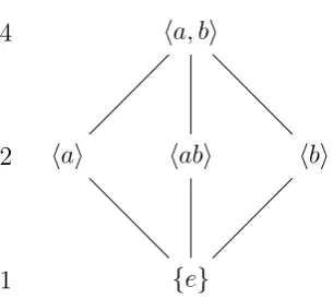
2
1
ha, bi
hai habi hbi
{e}
Figure 2.1: The graphical representation of the subgroup lattice forC2×C2. Each node shows the subgroups; The inclusion relations as subgroups are denoted by edges. The column of the numbers in the left side of the graph are the orders of the subgroups.
4
2
1
Q
Q(
√
2) Q(√6) Q(√3)
Q(
√
2,√3)
Figure 2.2: The graphical representation of the subfields that are fixed by the subgroups of C2×C2. Observe that this is the same graph as is presented for the subgroups. Each subfield is fixed by the Galois group situated at the corresponding node of the graph.
Let us consider another example: g = x4+x3+x2 + 1. It has four roots α, β =
α2, γ=α4=−α3−α2−α−1, δ=α3. We can construct four operations which permute the roots and construct the group C4. They are given by
e : α−→α (Identity)
a : α−→γ (1,2,3,4)
a2 : α−→β (1,3)(2,4)
4
2
1
hai
ha2i
{e}
Figure 2.3: The graphical representation of the subgroup lattice for C4. Each node shows the subgroups; The inclusion relations as subgroups are denoted by edges. The column of the numbers in the left side of the graph are the orders of the subgroups.
• InQ, the polynomial does not split.
• In Q(y), namely, in the extension by y such that y2+y−1 = 0, the polynomial splits into (x2−yx+ 1)(x2+ (y+ 1)x+ 1).
• InQ(α), the polynomial splits as (x−α)(x−β)(x−γ)(x−δ).
These examples are of the incorporation of the fundamental theorem of Galois theory.
Theorem 2.1. (FUNDAMENTAL THEOREM OF GALOIS THEORY) Let E be a Galois extension of F with Galois group G(which is denoted by Gal(E/F). There is a one-to-one correspondence between these two sets.
• The set of subgroups of G
• The set of sub-extensions ofF ⊂M ⊂E
• LetEH be the subfield corresponding to the subgroupH of Gal(E/F). EH is the set of elements of E which are fixed by every automorphism inH.
• H1 ⊃H2 ⇐⇒EH2 ⊃EH1.
• (H1:H2) = [EH2 :EH1]: the index of the subgroup and the degree of the extension is equal in the correspondence of the subgroups and subfields.
• For the automorphismσinF,EσHσ−1 =σ(EH), and, Gal(E/σM) =σGal(E/M)σ−1.
• IfH is normal inG,EH is the normal extension ofF and Gal(EH/F)'G/H.
In the first example, the Galois group is C2 × C2 and the Galois extension is Q(
√
Remark 2.2. Here we should recall the basic definitions concerning the Galois theory.
An algebraic field extension is the pair of a field K and a larger field L
which containsK, being made by the addition of extra elements toK. Such a circumstance is denoted by L/K (L overK). L is aK-vector space and its dimension is called the degree of LoverK and denoted by [L:K].
A normal extension is an algebraic field extension L/K, in which every polynomial (irreducible overK) either has no root inLor splits completely into linear factors inL.
A separable extension is an algebraic field extension E/F, in which the minimal polynomial of α(∈ E) over F has distinct roots. For α, we might find the polynomials with coefficients inF, to whichαis a root. The minimal polynomial is of the minimal degrees among them. The conjugate roots of
α might not always lie inF.
A Galois extensionE/F is an extension which is normal and separable. E is a splitting field of a separable polynomial with coefficients inF.
Aut(E/F) (the automorphism inE which fixes each element of F) is called the Galois group ofE/F.
A prime p inK factors (decomposes) into the product of the prime ideals in an extensionLofK in this way: pOL=Pe11· · ·P
eg
g . wherePi∩ OK =p. When ei > 1, the prime pi is said to ramify in L. Let n be the degree of
L overK, and let fi be the degree of the residue field extension ([OL/Pi :
O/p]). Thene1f1+· · ·egfg = [L:K]. In the case of Galois extension, the splitting occurs in this way: p= (B1· · ·Bg)e, withn=ef g.
An extensionLof a number field K is said to be unramified overK if there is no prime ideal ofOK which ramifies inOL.
A local field is the field which has a unique maximal ideal. (Caveat: for a field to be local, it requires more detailed conditions.) An extension L/K
of local fields is unramified if [L:K] = [OL/P:OK/p] where B (resp. p) is the maximal ideal ofL (resp.) K. In this case, the ramification index is
e= 1.
3
Exemplar computations by model molecules
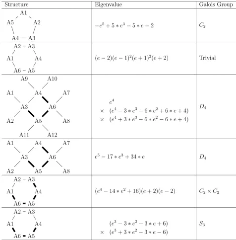
Structure Eigenvalue Galois Group A1 A2 A3 A4 A5
−e5+ 5∗e3−5∗e−2 C2
A1
A2 A3
A4
A5 A6
(e−2)(e−1)2(e+ 1)2(e+ 2) Trivial
A1 A2 A3 A4 A6 A5 A7 A8 A9 A10 A11 A12 e4
× (e4−3∗e3−6∗e2+ 6∗e+ 4)
× (e4+ 3∗e3−6∗e2−6∗e+ 4)
D4 A1 A2 A3 A4 A6 A5 A7 A8
e5−17∗e3+ 34∗e D
4 A1 A2 A3 A4 A5 A6
(e4−14∗e2+ 16)(e+ 2)(e−2) C 2×C2
A1
A2 A3
A4
A5 A6
(e3−3∗e2−3∗e+ 6)
× (e3+ 3∗e2−3∗e−6)
S3
Table 3.1: The model molecules to be examined in the study. In the rows, the structures are graphically represented, and along with them, the determinant of H−eI and the corresponding Galois group are given. The widths of the segments of the molecular models distinguish the strength of the electron hopping: Hij= -1 at thin ones; -2 at thick ones; if not connected, no interaction.
can analyze the determinant and the polynomials in the ideals, which are derived from the secular equations. We shall study some of them: those of pentagon and hexagon, and a molecule with the Galois group D4. The results of others are shown in the appendix (the supplemental part of the article). If one would get acquainted with the way to study the polynomials by computer algebra through these three chosen examples, it is easy to practice the analysis for others.
3.1
Simple model structures: two types of Galois group
of
C
2and the trivial one.
A1 A2 A3 A4
A5
Figure 3.1: The framework of a molecule of pentagonal structure. The atoms are indexed as A1,...,A5 and they interact between nearest neighbors, as are indicated by the bonds.
A1 A2 A3 A4 A5
A6
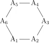
Figure 3.2: The framework of a hexagonal molecule. The atoms are indexed as A1,...,A6.
Let us compute the simple model of molecules. We place one orbital at each site and assume the interaction between neighboring orbitals, connected by the bonds (which are indicated by broad segments).
For the pentagonal model molecule, the result is as follows.
N=5 (Matrix H) Five atoms. 0, -1, 0, 0, -1,
-1, 0, -1, 0, 0, 0, -1, 0, -1, 0, 0, 0, -1, 0, -1, -1, 0, 0, -1, 0
Defining Ideal -y(1)*e-y(2)-y(5), -y(1)-y(2)*e-y(3), -y(2)-y(3)*e-y(4), -y(3)-y(4)*e-y(5), -y(1)-y(4)-y(5)*e,
y(1)^2+y(2)^2+y(3)^2+y(4)^2+y(5)^2-1
The determinant of (H-eI) -e^5+5*e^3-5*e-2
Standard Basis _[1]=e^3+e^2-3*e-2
_[2]=5*y(5)^2*e^2-5*y(5)^2*e-5*y(5)^2-e^2+e+1 _[3]=y(4)*e^2-y(4)*e-y(4)-y(5)*e^2+y(5)*e+y(5) _[4]=10*y(4)^2-2*y(4)*y(5)*e^3+14*y(4)*y(5)*e
+2*y(4)*y(5)-y(5)^2*e^3+2*y(5)^2*e^2+9*y(5)^2+e-3 _[5]=y(3)+y(4)*e+y(5)
_[6]=y(2)+y(3)*e+y(4) _[7]=y(1)+y(4)+y(5)*e
Primary Ideal Decomposition [1]:
[1]: !Primary ideal _[1]=e^2-e-1
_[2]=10*y(4)^2+10*y(4)*y(5)*e+10*y(5)^2+e-3 _[3]=y(3)+y(4)*e+y(5)
_[4]=y(2)-y(4)*e-y(5)*e^2+y(5) _[5]=y(1)+y(4)+y(5)*e
[2]: !Corresponding prime ideal. _[1]=e^2-e-1
_[2]=10*y(4)^2+10*y(4)*y(5)*e+10*y(5)^2+e-3 _[3]=y(3)+y(4)*e+y(5)
[2]: [1]:
_[1]=e+2
_[2]=5*y(5)^2-1 _[3]=y(4)-y(5)
_[4]=y(3)+y(4)*e+y(5)
_[5]=y(2)-y(4)*e-y(5)*e^2+y(5) _[6]=y(1)+y(4)+y(5)*e
[2]:
_[1]=e+2
_[2]=5*y(5)^2-1 _[3]=y(4)-y(5)
_[4]=y(3)+y(4)*e+y(5)
_[5]=y(2)-y(4)*e-y(5)*e^2+y(5) _[6]=y(1)+y(4)+y(5)*e
For the hexagonal model molecule, the result is as follows.
N=6 (Matrix H) Six atoms. 0, -1, 0, 0, 0, -1, -1, 0, -1, 0, 0, 0, 0, -1, 0, -1, 0, 0, 0, 0, -1, 0, -1, 0, 0, 0, 0, -1, 0, -1, -1, 0, 0, 0, -1, 0
Defining Ideal -y(1)*e-y(2)-y(6), -y(1)-y(2)*e-y(3), -y(2)-y(3)*e-y(4), -y(3)-y(4)*e-y(5), -y(4)-y(5)*e-y(6), -y(1)-y(5)-y(6)*e,
y(1)^2+y(2)^2+y(3)^2+y(4)^2+y(5)^2+y(6)^2-1
Standard Basis _[1]=e^4-5*e^2+4
_[2]=6*y(6)^2*e^2-6*y(6)^2-e^2+1
_[3]=2*y(5)*e^2-2*y(5)+y(6)*e^3-y(6)*e
_[4]=8*y(5)^2-2*y(5)*y(6)*e^5+9*y(5)*y(6)*e^3+
y(5)*y(6)*e-2*y(6)^2*e^4+12*y(6)^2*e^2-2*y(6)^2-2 _[5]=y(4)+y(5)*e+y(6)
_[8]=y(1)+y(5)+y(6)*e
Primary Ideal Decomposition [1]:
[1]:
_[1]=e-1
_[2]=4*y(5)^2+4*y(5)*y(6)+4*y(6)^2-1 _[3]=y(4)+y(5)*e+y(6)
_[4]=y(3)+1/2*y(6)*e^3-3/2*y(6)*e _[5]=y(2)-y(5)*e-y(6)*e^2+y(6) _[6]=y(1)+y(5)+y(6)*e
[2]:
_[1]=e-1
_[2]=4*y(5)^2+4*y(5)*y(6)+4*y(6)^2-1 _[3]=y(4)+y(5)*e+y(6)
_[4]=y(3)+1/2*y(6)*e^3-3/2*y(6)*e _[5]=y(2)-y(5)*e-y(6)*e^2+y(6) _[6]=y(1)+y(5)+y(6)*e
[2]: [1]:
_[1]=e+1
_[2]=4*y(5)^2-4*y(5)*y(6)+4*y(6)^2-1 _[3]=y(4)+y(5)*e+y(6)
_[4]=y(3)+1/2*y(6)*e^3-3/2*y(6)*e _[5]=y(2)-y(5)*e-y(6)*e^2+y(6) _[6]=y(1)+y(5)+y(6)*e
[2]:
_[1]=e+1
_[2]=4*y(5)^2-4*y(5)*y(6)+4*y(6)^2-1 _[3]=y(4)+y(5)*e+y(6)
_[4]=y(3)+1/2*y(6)*e^3-3/2*y(6)*e _[5]=y(2)-y(5)*e-y(6)*e^2+y(6) _[6]=y(1)+y(5)+y(6)*e
[3]: [1]:
_[1]=e+2
_[2]=6*y(6)^2-1 _[3]=y(5)-y(6)
_[4]=y(4)+y(5)*e+y(6)
_[5]=y(3)+1/2*y(6)*e^3-3/2*y(6)*e _[6]=y(2)-y(5)*e-y(6)*e^2+y(6) _[7]=y(1)+y(5)+y(6)*e
_[1]=e+2
_[2]=6*y(6)^2-1 _[3]=y(5)-y(6)
_[4]=y(4)+y(5)*e+y(6)
_[5]=y(3)+1/2*y(6)*e^3-3/2*y(6)*e _[6]=y(2)-y(5)*e-y(6)*e^2+y(6) _[7]=y(1)+y(5)+y(6)*e
[4]: [1]:
_[1]=e-2
_[2]=6*y(6)^2-1 _[3]=y(5)+y(6)
_[4]=y(4)+y(5)*e+y(6)
_[5]=y(3)+1/2*y(6)*e^3-3/2*y(6)*e _[6]=y(2)-y(5)*e-y(6)*e^2+y(6) _[7]=y(1)+y(5)+y(6)*e
[2]:
_[1]=e-2
_[2]=6*y(6)^2-1 _[3]=y(5)+y(6)
_[4]=y(4)+y(5)*e+y(6)
_[5]=y(3)+1/2*y(6)*e^3-3/2*y(6)*e _[6]=y(2)-y(5)*e-y(6)*e^2+y(6) _[7]=y(1)+y(5)+y(6)*e
Observe that in the case of the six-membered hexagonal model, the eigenvalues are obtained as integers, while in the case of the five-membered pentagonal model, some eigenvalues are unsolved and kept in a polynomial equation. To solve the equation, we should add an irrational number. In this case, the equation is given by
e2−e−1 = 0, (3)
to which, the solutions are
e1,2=
1±√5
2 . (4)
Let abe one of the roots of e2−e−1 = 0. In Q(a) =Q(
√
A:(y1(e1), y2(e1), y3(e1), y4(e1), y5(e1), e1) is defined by
e+ (a−1) = 0
10∗y(4)2+ (−10∗a+ 10)∗y(4)∗y(5) + 10∗y(5)2+ (−a−2) = 0
y(3) + (−a+ 1)∗y(4) +y(5) = 0
y(2) +y(3) + (a)∗y(5) = 0
y(1) +y(4) + (−a+ 1)∗y(5) = 0
B:(y1(e2), y2(e2), y3(e2), y4(e2), y5(e2)) is defined by
e+ (−a) = 0
10∗y(4)2+ (10∗a)∗y(4)∗y(5) + 10∗y(5)2+ (a−3) = 0
y(3) + (a)∗y(4) +y(5) = 0
y(2) +y(3) + (−a+ 1)∗y(5) = 0
y(1) +y(4) + (a)∗y(5) = 0
According to the Galois theory (as we have seen in the former section), the extension ofQevokes the automorphism, which fixes the polynomial equation with the coefficients inQ. The solutions A and B are interchangeable through the map
a←→1−a,
or, equivalently, √
5←→ −√5
3.2
Galois group
D
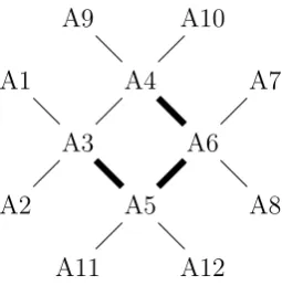
4A1
A2 A3
A4
A6
A5
A7
A8
A9 A10
A11 A12
Figure 3.3: A model molecule. The hopping integrals Hij are set to be −2 on the bonds denoted by broad edges; and Hij =−1 on others.
The result of the computation for this molecule is given below.
Matrix H
0, 0,-1, 0, 0, 0, 0, 0, 0, 0, 0, 0, 0, 0,-1, 0, 0, 0, 0, 0, 0, 0, 0, 0, -1,-1, 0,-1,-2, 0, 0, 0, 0, 0, 0, 0, 0, 0,-1, 0, 0,-2, 0, 0,-1,-1, 0, 0, 0, 0,-2, 0, 0,-2, 0, 0, 0, 0,-1,-1, 0, 0, 0,-2,-2, 0,-1,-1, 0, 0, 0, 0, 0, 0, 0, 0, 0,-1, 0, 0, 0, 0, 0, 0, 0, 0, 0, 0, 0,-1, 0, 0, 0, 0, 0, 0, 0, 0, 0,-1, 0, 0, 0, 0, 0, 0, 0, 0, 0, 0, 0,-1, 0, 0, 0, 0, 0, 0, 0, 0, 0, 0, 0, 0,-1, 0, 0, 0, 0, 0, 0, 0, 0, 0, 0, 0,-1, 0, 0, 0, 0, 0, 0, 0
The polynomial equation for spectra. [Determinant of H - e I]
e^12-21*e^10+80*e^8-84*e^6+16*e^4
Defining Ideal -y(1)*e-y(3), -y(2)*e-y(3),
-y(1)-y(2)-y(3)*e-y(4)-2*y(5), -y(3)-y(4)*e-2*y(6)-y(9)-y(10), -2*y(3)-y(5)*e-2*y(6)-y(11)-y(12), -2*y(4)-2*y(5)-y(6)*e-y(7)-y(8), -y(6)-y(7)*e,
-y(4)-y(9)*e, -y(4)-y(10)*e, -y(5)-y(11)*e, -y(5)-y(12)*e,
y(1)^2+y(2)^2+y(3)^2+y(4)^2+y(5)^2+y(6)^2+y(7)^2 +y(8)^2+y(9)^2+y(10)^2+y(11)^2+y(12)^2-1
Standard Basis
_[1]=e^9-21*e^7+80*e^5-84*e^3+16*e
_[2]=70176*y(12)^2*e+97*e^7-2059*e^5+8266*e^3-11608*e _[3]=8*y(11)+y(12)*e^8-21*y(12)*e^6+80*y(12)*e^4
-84*y(12)*e^2+8*y(12)
_[4]=24*y(10)*e+y(12)*e^7-21*y(12)*e^5+76*y(12)*e^3-36*y(12)*e _[5]=48*y(9)+48*y(10)+9*y(12)*e^8-185*y(12)*e^6+636*y(12)*e^4
-452*y(12)*e^2
_[6]=12*y(8)*e+y(12)*e^8-20*y(12)*e^6+61*y(12)*e^4-38*y(12)*e^2 _[7]=6*y(7)+6*y(8)+y(12)*e^7-20*y(12)*e^5+61*y(12)*e^3-38*y(12)*e _[8]=12*y(6)-y(12)*e^8+20*y(12)*e^6-61*y(12)*e^4+38*y(12)*e^2 _[9]=y(5)+y(12)*e
_[10]=24*y(4)-y(12)*e^7+21*y(12)*e^5-76*y(12)*e^3+36*y(12)*e _[11]=48*y(3)+y(12)*e^8-17*y(12)*e^6+4*y(12)*e^4+76*y(12)*e^2 _[12]=48*y(2)*e-y(12)*e^8+17*y(12)*e^6-4*y(12)*e^4-76*y(12)*e^2 _[13]=1376*y(2)^2+1376*y(8)^2+1376*y(10)^2+1376*y(12)^2
-e^8+23*e^6-126*e^4+336*e^2-688
_[14]=24*y(1)+24*y(2)-y(12)*e^7+17*y(12)*e^5-4*y(12)*e^3-76*y(12)*e
Primary Ideal Decomposition [1]:
[1]: !Primary ideal _[1]=e
_[2]=2*y(2)^2+2*y(8)^2+2*y(10)^2+2*y(12)^2-1
_[3]=y(11)+1/8*y(12)*e^8-21/8*y(12)*e^6+10*y(12)*e^4 -21/2*y(12)*e^2+y(12)
_[4]=y(9)+y(10)+3/16*y(12)*e^8-185/48*y(12)*e^6 +53/4*y(12)*e^4-113/12*y(12)*e^2
_[5]=y(7)+y(8)+1/6*y(12)*e^7-10/3*y(12)*e^5 +61/6*y(12)*e^3-19/3*y(12)*e
_[6]=y(6)-1/12*y(12)*e^8+5/3*y(12)*e^6 -61/12*y(12)*e^4+19/6*y(12)*e^2 _[7]=y(5)+y(12)*e
_[8]=y(4)-1/24*y(12)*e^7+7/8*y(12)*e^5-19/6*y(12)*e^3+3/2*y(12)*e _[9]=y(3)+1/48*y(12)*e^8-17/48*y(12)*e^6+1/12*y(12)*e^4
_[10]=y(1)+y(2)-1/24*y(12)*e^7+17/24*y(12)*e^5 -1/6*y(12)*e^3-19/6*y(12)*e
[2]: !Corresponding prime ideal _[1]=e
_[2]=2*y(2)^2+2*y(8)^2+2*y(10)^2+2*y(12)^2-1
_[3]=y(11)+1/8*y(12)*e^8-21/8*y(12)*e^6+10*y(12)*e^4 -21/2*y(12)*e^2+y(12)
_[4]=y(9)+y(10)+3/16*y(12)*e^8-185/48*y(12)*e^6 +53/4*y(12)*e^4-113/12*y(12)*e^2
_[5]=y(7)+y(8)+1/6*y(12)*e^7-10/3*y(12)*e^5 +61/6*y(12)*e^3-19/3*y(12)*e
_[6]=y(6)-1/12*y(12)*e^8+5/3*y(12)*e^6-61/12*y(12)*e^4 +19/6*y(12)*e^2
_[7]=y(5)+y(12)*e
_[8]=y(4)-1/24*y(12)*e^7+7/8*y(12)*e^5-19/6*y(12)*e^3 +3/2*y(12)*e
_[9]=y(3)+1/48*y(12)*e^8-17/48*y(12)*e^6+1/12*y(12)*e^4 +19/12*y(12)*e^2
_[10]=y(1)+y(2)-1/24*y(12)*e^7+17/24*y(12)*e^5 -1/6*y(12)*e^3-19/6*y(12)*e
[2]: [1]:
_[1]=e^4+3*e^3-6*e^2-6*e+4
_[2]=5848*y(12)^2+54*e^3+209*e^2-205*e-766
_[3]=4*y(10)+y(12)*e^3+3*y(12)*e^2-4*y(12)*e-2*y(12) _[4]=y(8)-y(12)
_[5]=4*y(2)+y(12)*e^3+3*y(12)*e^2-4*y(12)*e-2*y(12) _[6]=y(11)+1/8*y(12)*e^8-21/8*y(12)*e^6+10*y(12)*e^4 -21/2*y(12)*e^2+y(12)
_[7]=y(9)+y(10)+3/16*y(12)*e^8-185/48*y(12)*e^6 +53/4*y(12)*e^4-113/12*y(12)*e^2
_[8]=y(7)+y(8)+1/6*y(12)*e^7-10/3*y(12)*e^5+61/6*y(12)*e^3 -19/3*y(12)*e
_[9]=y(6)-1/12*y(12)*e^8+5/3*y(12)*e^6-61/12*y(12)*e^4 +19/6*y(12)*e^2
_[10]=y(5)+y(12)*e
_[11]=y(4)-1/24*y(12)*e^7+7/8*y(12)*e^5-19/6*y(12)*e^3 +3/2*y(12)*e
_[12]=y(3)+1/48*y(12)*e^8-17/48*y(12)*e^6+1/12*y(12)*e^4 +19/12*y(12)*e^2
_[13]=y(1)+y(2)-1/24*y(12)*e^7+17/24*y(12)*e^5 -1/6*y(12)*e^3-19/6*y(12)*e
_[1]=e^4+3*e^3-6*e^2-6*e+4
_[2]=5848*y(12)^2+54*e^3+209*e^2-205*e-766
_[3]=4*y(10)+y(12)*e^3+3*y(12)*e^2-4*y(12)*e-2*y(12) _[4]=y(8)-y(12)
_[5]=4*y(2)+y(12)*e^3+3*y(12)*e^2-4*y(12)*e-2*y(12) _[6]=y(11)+1/8*y(12)*e^8-21/8*y(12)*e^6+10*y(12)*e^4
-21/2*y(12)*e^2+y(12)
_[7]=y(9)+y(10)+3/16*y(12)*e^8-185/48*y(12)*e^6 +53/4*y(12)*e^4-113/12*y(12)*e^2
_[8]=y(7)+y(8)+1/6*y(12)*e^7-10/3*y(12)*e^5 +61/6*y(12)*e^3-19/3*y(12)*e
_[9]=y(6)-1/12*y(12)*e^8+5/3*y(12)*e^6 -61/12*y(12)*e^4+19/6*y(12)*e^2 _[10]=y(5)+y(12)*e
_[11]=y(4)-1/24*y(12)*e^7+7/8*y(12)*e^5-19/6*y(12)*e^3 +3/2*y(12)*e
_[12]=y(3)+1/48*y(12)*e^8-17/48*y(12)*e^6+1/12*y(12)*e^4 +19/12*y(12)*e^2
_[13]=y(1)+y(2)-1/24*y(12)*e^7+17/24*y(12)*e^5 -1/6*y(12)*e^3-19/6*y(12)*e
[3]: [1]:
_[1]=e^4-3*e^3-6*e^2+6*e+4
_[2]=5848*y(12)^2-54*e^3+209*e^2+205*e-766
_[3]=4*y(10)-y(12)*e^3+3*y(12)*e^2+4*y(12)*e-2*y(12) _[4]=y(8)+y(12)
_[5]=4*y(2)+y(12)*e^3-3*y(12)*e^2-4*y(12)*e+2*y(12) _[6]=y(11)+1/8*y(12)*e^8-21/8*y(12)*e^6+10*y(12)*e^4
-21/2*y(12)*e^2+y(12)
_[7]=y(9)+y(10)+3/16*y(12)*e^8-185/48*y(12)*e^6 +53/4*y(12)*e^4-113/12*y(12)*e^2
_[8]=y(7)+y(8)+1/6*y(12)*e^7-10/3*y(12)*e^5+61/6*y(12)*e^3 -19/3*y(12)*e
_[9]=y(6)-1/12*y(12)*e^8+5/3*y(12)*e^6-61/12*y(12)*e^4 +19/6*y(12)*e^2
_[10]=y(5)+y(12)*e
_[11]=y(4)-1/24*y(12)*e^7+7/8*y(12)*e^5-19/6*y(12)*e^3 +3/2*y(12)*e
_[12]=y(3)+1/48*y(12)*e^8-17/48*y(12)*e^6+1/12*y(12)*e^4 +19/12*y(12)*e^2
_[13]=y(1)+y(2)-1/24*y(12)*e^7+17/24*y(12)*e^5 -1/6*y(12)*e^3-19/6*y(12)*e
_[1]=e^4-3*e^3-6*e^2+6*e+4
_[2]=5848*y(12)^2-54*e^3+209*e^2+205*e-766
_[3]=4*y(10)-y(12)*e^3+3*y(12)*e^2+4*y(12)*e-2*y(12) _[4]=y(8)+y(12)
_[5]=4*y(2)+y(12)*e^3-3*y(12)*e^2-4*y(12)*e+2*y(12) _[6]=y(11)+1/8*y(12)*e^8-21/8*y(12)*e^6+10*y(12)*e^4
-21/2*y(12)*e^2+y(12)
_[7]=y(9)+y(10)+3/16*y(12)*e^8-185/48*y(12)*e^6 +53/4*y(12)*e^4-113/12*y(12)*e^2
_[8]=y(7)+y(8)+1/6*y(12)*e^7-10/3*y(12)*e^5 +61/6*y(12)*e^3-19/3*y(12)*e
_[9]=y(6)-1/12*y(12)*e^8+5/3*y(12)*e^6-61/12*y(12)*e^4 +19/6*y(12)*e^2
_[10]=y(5)+y(12)*e
_[11]=y(4)-1/24*y(12)*e^7+7/8*y(12)*e^5 -19/6*y(12)*e^3+3/2*y(12)*e
_[12]=y(3)+1/48*y(12)*e^8-17/48*y(12)*e^6 +1/12*y(12)*e^4+19/12*y(12)*e^2
_[13]=y(1)+y(2)-1/24*y(12)*e^7+17/24*y(12)*e^5 -1/6*y(12)*e^3-19/6*y(12)*e
We can reshape the decomposed components so that they should bereduced. Besides, we can compute the dimensions of them. The reshaped primary (indeed prime) ideals P1, P2, and P3 are given below. The ideal P1 is of dimension 3, and P1 and P2 are of dimension 0. Hence the ideal P1 delineates an object (an algebraic variety) of dimension 3 in the affine spaceQ[y(1), ..., y(12), e]; from which we can choose four representatives of the orthonormalized quantum states (at the spectrum e=0), with degeneracy 4, as is suggested by the determinant of H−eI. On the other hand, the ideal P2 and P3 delineate the algebraic varieties of dimension 0, which are the isolated points, and we choose one representative of the quantum state respectively.
P1=
(e, y(11)+y(12),y(9)+y(10),y(7)+y(8), y(6),y(5),y(4),y(3),
2*y(2)^2+2*y(8)^2+2*y(10)^2+2*y(12)^2-1, y(1)+y(2))
dim(P1)=3
P2=
(e^4+3*e^3-6*e^2-6*e+4,
5848*y(12)^2+54*e^3+209*e^2-205*e-766, y(11)-y(12),
y(8)-y(12), y(7)-y(12), y(6)+y(12)*e, y(5)+y(12)*e, 2*y(4)-y(12)*e^2-2*y(12)*e+2*y(12), 2*y(3)-y(12)*e^2-2*y(12)*e+2*y(12), 4*y(2)+y(12)*e^3+3*y(12)*e^2-4*y(12)*e-2*y(12), 4*y(1)+y(12)*e^3+3*y(12)*e^2-4*y(12)*e-2*y(12)) dim(P2)=0 P3=(e^4-3*e^3-6*e^2+6*e+4, 5848*y(12)^2-54*e^3+209*e^2+205*e-766, y(11)-y(12), 4*y(10)-y(12)*e^3+3*y(12)*e^2+4*y(12)*e-2*y(12), 4*y(9)-y(12)*e^3+3*y(12)*e^2+4*y(12)*e-2*y(12), y(8)+y(12), y(7)+y(12), y(6)-y(12)*e, y(5)+y(12)*e, 2*y(4)+y(12)*e^2-2*y(12)*e-2*y(12), 2*y(3)-y(12)*e^2+2*y(12)*e+2*y(12), 4*y(2)+y(12)*e^3-3*y(12)*e^2-4*y(12)*e+2*y(12), 4*y(1)+y(12)*e^3-3*y(12)*e^2-4*y(12)*e+2*y(12)) dim(P3)=0
The decomposed ideals could split more if we place them in the extension field in which the univariate polynomials of the variable ’e’ shall split.
Let us take one of the components in the primary ideal decomposition and inspect the Galois correspondence. For the component P2, the eigenvalues are the root of this polynomial:
f =x4+ 3x3−6x2−6x+ 4.
The Galois group of the polynomial is D4. In this case, therefore, it is sufficient to use the extension field with the Galois groupD4.
Remark 3.1. It is not trivial how to determine the Galois group; The book by Milne [Mil18] explains how to do it, and computer algebra programs [PARI/GP [The19] and GAP [The17]] can compute it.
The roots of the equation are given by
x = − q
3√17
2 + 29 2 2 − √ 17 4 , q
3√17
2 + 29 2 2 − √ 17 4 , √ 17 4 − q 29 2 −
3√17 2 2 , √ 17 4 + q 29 2 −
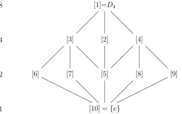
The Galois extension for D4 is illustrated in Fig. 3.4. The group D4 contains 9 subgroups and there are two pairs of conjugated subgroups.
8
4
2
1
[1]=D4
[3] [2] [4]
[6] [7] [5] [8] [9]
[10] ={e}
Figure 3.4: The graphical representation of the subgroup lattice for D4. Each node shows the subgroups; The inclusion relations as subgroups are denoted by edges. Two pairs of subgroups ([6] and [7], [8] and [9]) are conjugated in the same classes. The column of the numbers in the left side of the graph are the orders of the subgroups.
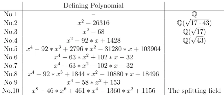
Let us analyze the equation using PARI/GP. A short computer program is presented in the appendix E. At first one should prepare the splitting field off to study the Galois extension. Usually one has only to add four distinct roots toQto generate it. However, the splitting field proposed by PARI/GP is not of this kind, as the defining polynomial is
K =x8−46∗x6+ 461∗x4−1360∗x2+ 1156.
This polynomial is different to f, although the Galois group operation in the splitting field forK shall evolve the permutation of four roots off. In addition, the Galois group of this polynomial isD4. The use of the alternative polynomialK makes the treatment simpler, as the splitting field of f is constructed by the addition of only one of the root of the polynomialK toQ.
Defining Polynomial
No.1 – Q
No.2 x2−26316
Q(
√
17·43)
No.3 x2−68
Q(
√
17)
No.4 x2−92∗x+ 1428 Q(√43)
No.5 x4−92∗x3+ 2796∗x2−31280∗x+ 103904 No.6 x4−63∗x2+ 102∗x−32
No.7 x4−63∗x2−102∗x−32
No.8 x4−92∗x3+ 1844∗x2−10880∗x+ 18496
No.9 x4−58∗x2+ 153
No.10 x8−46∗x6+ 461∗x4−1360∗x2+ 1156 The splitting field
Table 3.2: The list of subfields in the Galois extension. One can construct each of them by adding one of the roots of the defining polynomial toQ.
In these subfields, the polynomial equationffor the spectrum e splits in the following way. All polynomials share the four common roots, indexed by 1, 2, 3, and 4. The number-lists between the square brackets stand for the roots given by this index.
NO.1
(1) x^4 + 3*x^3 - 6*x^2 - 6*x + 4 [1,2,3,4]
---NO.2
(2) x^4 + 3*x^3 - 6*x^2 - 6*x + 4 [1,2,3,4]
---NO.3
(1) x^2 + Mod(-1/4*y + 3/2, y^2 - 68)*x - 2 [1,4] (2) x^2 + Mod(1/4*y + 3/2, y^2 - 68)*x - 2 [2,3]
---NO.4
(1) x^4 + 3*x^3 - 6*x^2 - 6*x + 4 [1,2,3,4]
---NO.5
(1) x^2 + Mod(-1/620*y^3 + 69/620*y^2 - 11/5*y + 1992/155, y^4 - 92*y^3 + 2796*y^2 - 31280*y + 103904)*x - 2 [1,4]
---NO.6
(1) x + Mod(-2/49*y^3 - 3/98*y^2 + 213/98*y - 69/49, y^4 - 63*y^2 + 102*y - 32) [1]
(2) x + Mod(6/49*y^3 + 9/98*y^2 - 737/98*y + 354/49, y^4 - 63*y^2 + 102*y - 32) [4]
(3) x^2 + Mod(-4/49*y^3 - 3/49*y^2 + 262/49*y - 138/49, y^4 - 63*y^2 + 102*y - 32)*x - 2 [2,3]
---NO.7
(1) x + Mod(-6/49*y^3 + 9/98*y^2 + 737/98*y + 354/49, y^4 - 63*y^2 - 102*y - 32) [3]
(2) x + Mod(2/49*y^3 - 3/98*y^2 - 213/98*y - 69/49, y^4 - 63*y^2 - 102*y - 32) [2]
(3) x^2 + Mod(4/49*y^3 - 3/49*y^2 - 262/49*y - 138/49, y^4 - 63*y^2 - 102*y - 32)*x - 2 [1,4]
---NO.8
(1) x^2 + Mod(-5/6528*y^3 + 247/3264*y^2 - 725/408*y + 119/12, y^4 - 92*y^3 + 1844*y^2 - 10880*y + 18496)*x
+ Mod(-7/1088*y^3 + 305/544*y^2 - 156/17*y + 55/2,
y^4 - 92*y^3 + 1844*y^2 - 10880*y + 18496) [3,4] (2) x^2 + Mod(5/6528*y^3 - 247/3264*y^2 + 725/408*y - 83/12,
y^4 - 92*y^3 + 1844*y^2 - 10880*y + 18496)*x [1,2] + Mod(-3/2176*y^3 + 121/1088*y^2 - 197/136*y + 17/4,
y^4 - 92*y^3 + 1844*y^2 - 10880*y + 18496)
---NO.9
(1) x^2 + Mod(-1/2*y + 3/2, y^4 - 58*y^2 + 153)*x
+ Mod(-1/24*y^3 + 1/8*y^2 + 49/24*y - 33/8, y^4 - 58*y^2 + 153) [1,3] (2) x^2 + Mod(1/2*y + 3/2, y^4 - 58*y^2 + 153)*x
+ Mod(1/24*y^3 + 1/8*y^2 - 49/24*y - 33/8, y^4 - 58*y^2 + 153) [2,4]
---NO.10
(1) x + Mod(5/1632*y^6 - 247/1632*y^4 + 725/408*y^2 - 1/2*y - 83/24, y^8 - 46*y^6 + 461*y^4 - 1360*y^2 + 1156) [1]
(3) x + Mod(-7/544*y^7 - 5/1632*y^6 + 305/544*y^5
+ 247/1632*y^4 - 78/17*y^3 - 725/408*y^2 + 55/8*y + 119/24, y^8 - 46*y^6 + 461*y^4 - 1360*y^2 + 1156) [3]
(4) x + Mod(7/544*y^7 - 5/1632*y^6 - 305/544*y^5 + 247/1632*y^4 + 78/17*y^3 - 725/408*y^2 - 55/8*y + 119/24,
y^8 - 46*y^6 + 461*y^4 - 1360*y^2 + 1156) [4]
---Notice that we use a special notation to represent the coefficients in the subfields: when a coefficient is given by modulo, say,
Mod(−1/4∗y+ 3/2, y2−68),
it implies a number−1/4y+ 3/2, defined byysuch thaty2−68 = 0. This is the notation adopted by PARI/GP.
One might feel the necessity to know in what way these irreducible polynomials in the subfields encapsulate the four root of the polynomialf. We can check it after some algebra as follows.
• LetQ(a) is the splitting field ofK.
• For each subfield ofQ(a), its defining polynomial splits in Q(a). The rootsβi are given by polynomialsβi(a).
• The polynomial f splits into the set of polynomials in the subfields. The latter polynomials have the coefficients composed of ’y’ which is one of the roots of the defining polynomial of the subfield.
• By the substitutiony→βi(a) (with an availableβi) for these polynomials factor-ized in the subfield, we get the representations inQ(a) that split.
No.1 [ (1,2)(3,7)(4,6)(5,8), (1,7,6,5)(2,8,4,3) ]; [ a, b ]
No.2 [ (1,7,6,5)(2,8,4,3) ]; [ b ]
No.3 [ (1,2)(3,7)(4,6)(5,8), (1,6)(2,4)(3,8)(5,7) ]; [ a, b^-2 ]
No.4 [ (1,8)(2,7)(3,6)(4,5), (1,6)(2,4)(3,8)(5,7) ]; [ b^-1*a, b^-2 ]
No.5 [ (1,6)(2,4)(3,8)(5,7) ]; [ b^-2 ]
No.6 [ (1,2)(3,7)(4,6)(5,8) ]; [ a ]
No.7 [ (1,4)(2,6)(3,5)(7,8) ]; [ a*b^-2 ]
No.8 [ (1,8)(2,7)(3,6)(4,5) ]; [ b^-1*a ]
No.9 [ (1,3)(2,5)(4,7)(6,8) ]; [ a*b^-1 ]
No.10[ ( ) ]; [ e ]
Table 3.3: The Galois groups and the subgroups corresponding to the Galois extension, represented by the generators ofD4. (a2 =b4 =e, ab=b−1a).
Remark 3.2. If one would like to see the Galois group operations on the roots off, one should make use of the automorphisms of the splitting field. Let y be one of the roots of the polynomialK. The automorphism is composed of polynomials of y in this way:
y -> -y,
y -> -7/272*y^7 + 305/272*y^5 - 156/17*y^3 + 55/4*y,
y -> -7/544*y^7 - 5/816*y^6 + 305/544*y^5 + 247/816*y^4 - 78/17*y^3 - 725/204*y^2 + 59/8*y + 101/12,
y -> -7/544*y^7 + 5/816*y^6 + 305/544*y^5 - 247/816*y^4 - 78/17*y^3 + 725/204*y^2 + 59/8*y - 101/12,
y -> 7/544*y^7 - 5/816*y^6 - 305/544*y^5 + 247/816*y^4 + 78/17*y^3 - 725/204*y^2 - 59/8*y + 101/12,
y -> 7/544*y^7 + 5/816*y^6 - 305/544*y^5 - 247/816*y^4 +78/17*y^3 + 725/204*y^2 - 59/8*y - 101/12,
y -> 7/272*y^7 - 305/272*y^5 + 156/17*y^3- 55/4*y
In the next section, we shall discuss more the significance of the result presented in this section.
4
Review of the computation
4.1
From the simple model to the realistic system
We have worked in the rational number field Q. However, in general cases, the matrix elements in the secular equations are real numbers and the corresponding polynomials have the coefficients of real numbers. Hence we should conduct the study not inQ, but in
Q({Hij},{Sij}),
that is an extension ofQ, to which the matrix elements{Hij}and{Sij}are added. One could extend this field and study the equations involved therein using the Galois theory. Notice that it is not obligatory to compute in the field of real numbers;{Hij}and {Sij}
might be replaced with the approximations with rational numbers; then one can work inQ.
4.2
Quantum mechanics as the objects of number theory
In this section, we make a review of the computation executed hitherto. As the eigen-states of quantum mechanics are represented by polynomials, one may expect the split-ting of polynomial ideals in the extension of the fields, as is customary in the number theory:
p=Pe1
1 P e2
Let us see how the splitting occurs. When the monomial order (for the Gr¨obner bases) is properly chosen, we obtain the set of polynomials to which the variables are added one by one. An example of this is the idealp which we have obtained in the exemplary computation of a model molecule with the Galois group D4. The generators of p are given below.
_[1]=e^4+3*e^3-6*e^2-6*e+4
_[2]=5848*y(12)^2+54*e^3+209*e^2-205*e-766
_[3]=4*y(10)+y(12)*e^3+3*y(12)*e^2-4*y(12)*e-2*y(12) _[4]=y(8)-y(12)
_[5]=4*y(2)+y(12)*e^3+3*y(12)*e^2-4*y(12)*e-2*y(12) _[6]=y(11)+1/8*y(12)*e^8-21/8*y(12)*e^6+10*y(12)*e^4
-21/2*y(12)*e^2+y(12)
_[7]=y(9)+y(10)+3/16*y(12)*e^8-185/48*y(12)*e^6 +53/4*y(12)*e^4-113/12*y(12)*e^2
_[8]=y(7)+y(8)+1/6*y(12)*e^7-10/3*y(12)*e^5 +61/6*y(12)*e^3-19/3*y(12)*e
_[9]=y(6)-1/12*y(12)*e^8+5/3*y(12)*e^6 -61/12*y(12)*e^4+19/6*y(12)*e^2 _[10]=y(5)+y(12)*e
_[11]=y(4)-1/24*y(12)*e^7+7/8*y(12)*e^5-19/6*y(12)*e^3 +3/2*y(12)*e
_[12]=y(3)+1/48*y(12)*e^8-17/48*y(12)*e^6+1/12*y(12)*e^4 +19/12*y(12)*e^2
_[13]=y(1)+y(2)-1/24*y(12)*e^7+17/24*y(12)*e^5 -1/6*y(12)*e^3-19/6*y(12)*e
If the polynomial for the energy spectrum, given at first as [1], is split, we can decompose the corresponding algebraic variety into four subsets:
V(p) =V(P1)∪V(P2)∪V(P3)∪V(P4) where the subsets are defined by four idealsPi(i= 1, ...,4) such that
p=P1∩P2∩P3∩P4
Observe that the representation concerning the decomposition is given by the intersec-tion; but the intersection is replaced with the product, as the four decomposed ideals are coprime with each other. (Recall the definition: two ideals a and b are coprime if and only ifa+b= (1); for such a pair,a·b=a∩b.) These four ideals are obtained only by replacing the first polynomial by a linear one:
e−αi.
φ1
φ2 φ3
φ4
φ1 = (e−α1,264∗y(6)2−5∗e2+ 2,4∗y(5)−y(6)∗e3+ 14∗y(6)∗e, ...) φ2 = (e−α2,264∗y(6)2−5∗e2+ 2,4∗y(5)−y(6)∗e3+ 14∗y(6)∗e, ...) φ3 = (e−α3,264∗y(6)2−5∗e2+ 2,4∗y(5)−y(6)∗e3+ 14∗y(6)∗e, ...) φ4 = (e−α4,264∗y(6)2−5∗e2+ 2,4∗y(5)−y(6)∗e3+ 14∗y(6)∗e, ...)
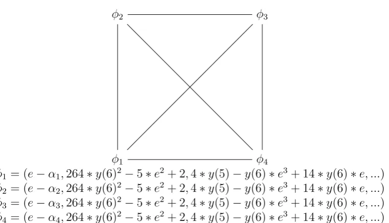
Figure 4.1: The permutation of the quantum states induced by the extension of field.
Let us clarify the points.
• The prime ideal p in Q contains the polynomial of four degrees PE, univariate of the variable of the energy spectrum. In the splitting field, it splits into four linear polynomials, and the ideal also splits into four prime ideals. As the other variables are linking to the energy spectrum ’e’, the automorphism, (namely, the permutation of the roots of that equation) causes the permutation of the four prime ideals.
• In the splitting field, the four ideals that represent four quantum states are conju-gate. In the subfields, these ideals would merge into prime ideals that encapsulate several quantum states.
• It is easy to write down the generators of prime ideals in the subfields. We have the prime idealpin the base ring, andphas the univariate polynomialpE which gives the energy spectra. In the subfields, this polynomialpE shall split into qE1 · · ·q
g E, as is demonstrated in the preceding section. In the generating set ofp, we replace
pE with any of qE1, ..., q g
E to make the set of prime idealsP1, ...Pg in the subfield.
• Consider the prime ideals in one subfield. The operation of the subgroups permutes the conjugate pair of the quantum states belonging to the same prime ideal. And it does not intermingle the quantum states between represented by different prime ideals. On the other hand, if the subgroupN is normal in the Galois groupG, the factor groupG/N shall permute the quantum states belonging to different prime ideals.
8
4
2
1
(p)
P3,1P3,2 P2 P4
P6,1P6,2P6,3 P7,1P7,2P7,3 P5,1P5,2 P8,1P8,2 P9,1P9,2
P10,1P10,2P10,3P10,4
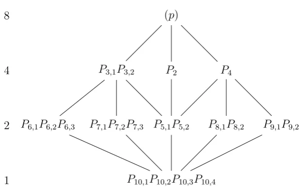
Figure 4.2: The graphical representation of the splitting of the ideals D4. Each node stands for the subfield, upon which transcribed are the factorized prime ideals enclosing quantum states. The inclusion relations as subfields are denoted by edges. The column of the numbers in the left side of the graph are the degrees of extensions.
The model molecule under investigation has two prime ideals other thanpinQ[y(1), ..., y(12), e] Let us go back to Section 3.2 and ascertain what they are. According to the list in that
section, the firstp1 is of dimension 3 with spectrume= 0; the secondp2 ispused above; the third p3 is of dimension 0 with spectra e4−3e3−6e2+ 4 = 0. These three prime ideals are interchanged by an operation as follows.
e ←→ −e
p1 ←→ p1 p2 ←→ p3
The change of the sign of ’e’ fixesp1 while it interchangesp2 and p3. p3 is the replica of
p2, similarly under the action of the Galois groupD4.
amplitude of the wave function. The new labels are the roots of the univariate polynomial equation of y(i). The splitting field for this polynomial is larger than that for the polynomial of the energy spectrum. This is because of the double-fold degeneracy of y(i); indeed φ and −φ are equivalent quantum states from the viewpoint of quantum mechanics, although they are distinguishable in the algebraic variety.
We dare say there is a hidden symmetry, which originates from the automorphism of the number field. Traditionally we have analyzed the symmetry in molecules using the point group that acts upon the atomic configuration, which fixes the secular equation and the energy spectrum [Wey50, Tin03, DDJ08]. However, the Galois theory provides the quantum system with another sort of symmetry, as we have seen now. (We use the term symmetry, so long as group-theoretic operations mutate the wavefunctions.) The apparent difference is that the energy spectrum is not fixed but changeable through the automorphism of the extended field. Note that the quantum states, exchangeable by the Galois theoretic automorphism, are included in the same irreducible representations of the molecular point group because they satisfy the same set of equations.
Concerning the point group operation, one should keep in mind this: the residue ring by a 0-dimensional ideal is denoted by
Q[y1, y2, ..., yn, e]/p. It stands for a field
Q(α1, α2, ...αn, β),
where (α1, α2, ...αn, β) ∈ V(p). (That is to say, (α1, α2, ...αn, β) is the solution of the polynomial equations defined byp.) One can construct the automorphism of the former large field, which contains the point-group operation on the wavefunctions. In this wise, our exemplar computation is the study of the part of the automorphism in this field, as we have worked in Q(e) modestly. The unified modeling of the Galois group and the point group would be possible.
5
Class field theory and quantum mechanics
5.1
Preliminaries
The aim of class field theoryis to establish the correspondence between a type of group generated by ideals and the Galois group in the extension of the field [Mil17, Con01, AT68, Ser79, Gra13].
As we know, one of the fundamental items in number theory is the ideal, which is the set closed by the multiplication and the addition. Besides, in a similar way to the integers, the division between two ideals is defined. The consequence of this extension is the fractional ideal, in which a kind of group structure is built.
composed of the principal ideals inKwhich satisfy a certain condition. It is proved that the number of classes in a number field is limited.
In the extension field, the ideal class group and that of the Galois group are deeply re-lated; to establish the correspondence between these two objects is the principal concern of the class field theory.
To construct the class field theory, we have to define several things. Let L be a separable extension of degree n over K, withK-homomorphisms (σ1, ...σn). The rings of integers for these fields are denoted byOL and OK. The prime ideal inK is denoted by pand the prime ideal in Lthat divide pis denoted byB.
• [Ring of integer]An element of the field is F integral over Z if it satisfies the equation
xm+a1xm−1+·+am = 0,
witha1, ...am ∈Z. The ring of elements ofL integral over Zis called the integral closure ofZinL. The integral closure ofZin an algebraic number fieldLis called the ring of integersOL inL.
• [Trace and Norm] The trace and norm maps are defined in the following way. TrL/K(β) :=σ1(β) +· · ·σn+ (β); NmL/K :=σ1(β)× · · · ×σn(β)
• [Fractional ideal] A fractional ideal I in K is a set of elements such that there exists a non-zeror∈ OK and rI⊆ OK
• [Modulus] A modulus of a number field K is the formal product of ideals: m=
m0m∞, wherem0is the products of finite primes;m∞is that of infinite real primes. (The definition of the latter is complicated. It is a kind of sign condition which we use for the real numbers.) We denote by S(m) the set of prime ideals which dividem.
• [The group of fractional ideals with a modulus] Let IS be the group of fractional ideals generated the prime ideals of K which do not lie in S.
• [Ray class group] LetCm be the quotientIS(m)/i(Km,1). We defineKm,1 to be the set generated by the elementasuch that
ordp(a−1)≥ordp(m0) for all prime ideals pdividingm0, and,
ap >0
• [Frobenius map] Frobenius element, denoted by (P, L/K) is the unique elementσ
of Gal(L/K) satisfying the following two conditions:
σP=P
and for allα ∈OL
σ(α)≡αqmodP
where q is the number of elements the residue fieldOK/p. For an extensionL of
K, let S0(m) be the prime ideals of L lying over the prime ideals in S(m). We have a norm map Nm :IS0(m)→IS(m) such that Nm(P) =pf wherep=OK∩P. Letf is the residue class degree [OL/P:OK/p]. Then we have
(Nm(B), L/K) = (pf, L/K)def= (p, L/K)f = 1.
Hence Nm(IS0(m)) is contained in the kernel of IS(m)→Cm.
Theorem 5.1 (ARTIN, Reciprocity law). Let Lbe an abelian extension of K; let S be the set of prime ideals that ramify in L. For some modulus msuch that S(m) =S, the homomorphism
IS→Gal(L/K),
or,
p7→(p, L/K)
factors throughCm=IS(m)/i(Km,1). It induces an isomorphism
IS(m)/i(Km,1)·Nm(IS
0(m)
)→Gal(L/K)
whereS0(m) are the prime ideals ofL lying over the prime ideals inS(m. In particular, the prime ideals splitting in Lexactly belong to the subgroup of IS, given by
˜
H =i(Km,1)·Nm(IS
0(m)
).
Theorem 5.2 (LOCAL RECIPROCITY LAW). For every non-archimedean local field
K, there exists a unique homomorphism
φK :K× →Gal(Kab/K)
with the following properties:
(a) for every prime elementπ of K and every finite unramified extension L ofK,
φK(π) acts onL as the Frobenius map(FrobL/K);
(b) for every finite abelian extensionLofK, NmL/K(L×) is contained in the kernel ofa→φK(a)|L, and φK induces an isomorphism
φK :K×/NmL/K(L×)→Gal(L/K)
In particular, we have
K×: NmL/K(L×)
Let us denote NmL/K(L×) by Nm(L×). The statement (b) says that, for every finite abelian extension L of K, the map K factors as follows:
K× Gal(Kab/K)
K×/Nm(L×) Gal(L/K)
quotient map
φK
'
φL/K
τ 7→τ|L
In the above diagram, φK and φL/K are the local Artin maps (the local reciprocity maps) for K and L/K. φL/K is often called the norm residue map and denoted by
a7→(a, L/K). The subgroups ofK×, given by Nm(L×) for some finite abelian extension
L ofK, are called the norm groups in K.
Theorem 5.3 (EXISTENCE THEOREM). For every congruence subgroupH modulo
m, there exists a finite abelian extension L/K such thatH =i(Km,1)NmL/K(ILm). At a glance, it is unclear how to constitute a class field. However, This fact is affirmed.
• Every abelian extension of Q is a class field. (Another version of the statement goes as follows: according to the Kronecker-Weber theorem (the primitive version of the existence theorem), every abelian extension ofQis contained in a cyclotomic extension.
In the following sections, we execute heuristic computations to comprehend these concepts and statements.
5.2
Feasibility of class field theory in quantum mechanics
As far as we concern ourselves about the computation of quantum mechanics, which is accomplished by the decomposition of ideals, this sort of statement is quite touching for us. We use the prime idealspin the base ringR=Q[y1, ...yn, e] to represent a quantum state. If the polynomial representation is possible, anything related to this quantum state is given symbolically by the ideal I in the ring of integers of the quotient field
a polynomial. In class field theory, however, as the ray class group is the quotient of the group of fractional ideals by a certain class of principal ideals, there are principal ideals which reduce to the identity. Hence the observable as the principal ideal might be the trivial element in the class group, from which we could not expect any useful application. Then what shall be a non-principal ideal? In a sense, it is the line of mass production of mathematical objects from a set of generators. If one is engaged in a bunch of computations using the elements in an ideal I, the factorization of the ideal might economize the cost of computation, as it would serve as a kind of Karatsuba algorithm. However, it is not of the interest of quantum mechanics.
Besides, it seems that there would be technical difficulties to construct the class field for the polynomial algebra. One has to prove the existence of the maximum abelian extension that should be the class field. At the same time, one has to substantiate it by polynomials, establishing the maps between the class group and the Galois group. A far as the authors investigate the references, the existence of class field has been proven for the function field, as well as for the number field; for these two objects, the concrete construction of the class field should be possible. Hence the class field theory over the algebra of polynomials would be practicable. However, the general-purpose algorithm to build the class field seems to be unknown for the latter case.
If p is 0-dimensional, R/pR is an extension of Q and the class field theory might be applicable. However, this number field appears to be too large; it might not be an abelian extension. We know that the entries in the solutions of the equation p= 0 are mutually dependent, owing to the specific forms of the defining polynomials. (As for the dependence of the variables, review the generators of prime ideals given in Section 3.2.) However, once they are lifted to the extension field, such dependence is hardly discerned. We prefer to work on a smaller scale, always keeping in mind the feature of the polynomial ideal.
For these reasons, at present, we postpone the plan to construct the class field over the polynomial algebra. Instead, we seek another channel from which the outcome of class field theory could be conducted into quantum mechanics.
5.3
Consequence of class field theory in quantum
mechan-ics
Let us see a consequence of the theorem concerning the class field theory. In this section, we choose a model molecule with the Galois group C2×C2, the analysis of which is given in the appendix B. One of the entries of the primary ideal decomposition is given as follows.
P1=
(e^4-14*e^2+16, 264*y(6)^2-5*e^2+2,
4*y(3)+y(6)*e^3-12*y(6)*e, 2*y(2)-y(6)*e^2+12*y(6), 4*y(1)+y(6)*e^3-12*y(6)*e )
It contains four quantum states, distinguished by four energy spectra, which are the roots of the first univariate polynomial of the variable ’e’: e4−14e2+ 16. Let us compute the Galois extension and factorize the polynomial, using PARI/GP. We must recall these things: as we have seen, the factorization of the polynomial causes that of the ideal; the permutation of the roots of the polynomial is equivalent to that of the quantum states.
/* Define the polynomial f. */ f=Pol([1,0,-14,0,16])
/* Compute the splitting field and get the defining polynomial L*/ L=nfsplitting(f) /*In this case L=f */
nf=nfinit(L);
/* Make the Galois extension. */ gal=galoisinit(L);
Under the decomposition of the polynomial, the ideal P1 decomposes into P11, P12, P13, and P14 in the extension fieldL=Q(a), where ais a root of the polynomialf.
Let us try an experiment: choose a prime integer p (in Z) and decompose it in L. One finds the set of prime ideals (P[1]....P[g]) in Q(a) lying overp. Thereinp might be decomposed into the different numbers of prime ideals. From each of these prime ideals, one could manage to make the so-called Frobenius map, which has this property:
σ(x) ==x#N[p]modP[i],
where simply #N[p] =p for a prime. This is an automorphism inQ(a)/Q. (In general, for the extensionL overK, the Frobenius map is denoted by (P, L/K).) How it would be? Once it is built, it also acts as the transmuting map among the four quantum states P12, P12, P13, and P14.
Remark 5.1. The proof of the existence of the Frobenius element requires a short argument, as is given in Chapter 8 of [Mil17]. One can find the Frobenius element by symbolic computations.
Let us define a small function of PARI/GP.
procmakefrobenius(p)= {
prs=idealprimedec(nf,p);
g = vector(#prs,k,idealfrobenius(nf,gal,prs[k])); polmap=vector(#g,k,galoispermtopol(gal,g[k])); return(polmap);
The function does the prime ideal decomposition of the given prime number in the extension field; then, for each of the prime ideals obtained by the decomposition, it computes the Frobenius map. The result is a table, in which the Frobenius maps are transcribed. (Hence the length of the table is the number of the decomposed factors; it might be 1, 2, or 4.) Let us try the computation with the list of primes in Z. As the discriminant of the polynomial f is 4460504 = 212·32·11, the primes that shall ramify in Q(a) are only three: 2, 3, and 11. From these primes, one could not make the Frobenius map, and we omit them from the experiment. The result given below shows the primes and the corresponding Frobenius maps. The Frobenius maps are given by the polynomialsF rb(x), which maps the generator ’a’ ofQ(a) bya7→F rb(a). The permutations of the four roots of the polynomial f (viz., the permutation in four quantum states), induced by the Frobenius map, are also shown.
prime->[Frobenius maps]
5->[1/4*x^3 - 7/2*x, 1/4*x^3 - 7/2*x] !(1,2)(3,4) 7->[-1/4*x^3 + 7/2*x, -1/4*x^3 + 7/2*x] !(1,3)(2,4) 13->[-1/4*x^3 + 7/2*x, -1/4*x^3 + 7/2*x]
17->[-x, -x] !(1,4)(2,3) 19->[1/4*x^3 - 7/2*x, 1/4*x^3 - 7/2*x]
23->[1/4*x^3 - 7/2*x, 1/4*x^3 - 7/2*x]
29->[x, x, x, x] !() 31->[-x, -x]
37->[-x, -x] 41->[-x, -x]
43->[1/4*x^3 - 7/2*x, 1/4*x^3 - 7/2*x] 47->[1/4*x^3 - 7/2*x, 1/4*x^3 - 7/2*x] 53->[1/4*x^3 - 7/2*x, 1/4*x^3 - 7/2*x] 59->[-1/4*x^3 + 7/2*x, -1/4*x^3 + 7/2*x] 61->[-1/4*x^3 + 7/2*x, -1/4*x^3 + 7/2*x] 67->[x, x, x, x]
71->[1/4*x^3 - 7/2*x, 1/4*x^3 - 7/2*x] 73->[1/4*x^3 - 7/2*x, 1/4*x^3 - 7/2*x] 79->[-1/4*x^3 + 7/2*x, -1/4*x^3 + 7/2*x] 83->[-x, -x]
89->[-1/4*x^3 + 7/2*x, -1/4*x^3 + 7/2*x] 97->[x, x, x, x]
101->[x, x, x, x] 103->[-x, -x] 107->[-x, -x]
109->[-1/4*x^3 + 7/2*x, -1/4*x^3 + 7/2*x] 113->[-1/4*x^3 + 7/2*x, -1/4*x^3 + 7/2*x] 127->[-1/4*x^3 + 7/2*x, -1/4*x^3 + 7/2*x] 131->[-x, -x]
139->[1/4*x^3 - 7/2*x, 1/4*x^3 - 7/2*x] 149->[x, x, x, x]
151->[-1/4*x^3 + 7/2*x, -1/4*x^3 + 7/2*x] 157->[-x, -x]
163->[x, x, x, x] 167->[x, x, x, x] 173->[x, x, x, x]
179->[-1/4*x^3 + 7/2*x, -1/4*x^3 + 7/2*x] 181->[-x, -x]
191->[1/4*x^3 - 7/2*x, 1/4*x^3 - 7/2*x] 193->[1/4*x^3 - 7/2*x, 1/4*x^3 - 7/2*x] 197->[x, x, x, x]
199->[-x, -x]
211->[1/4*x^3 - 7/2*x, 1/4*x^3 - 7/2*x] 223->[-x, -x]
227->[-x, -x] 229->[-x, -x] 233->[-x, -x] 239->[x, x, x, x]
241->[1/4*x^3 - 7/2*x, 1/4*x^3 - 7/2*x] 251->[-1/4*x^3 + 7/2*x, -1/4*x^3 + 7/2*x] 257->[-1/4*x^3 + 7/2*x, -1/4*x^3 + 7/2*x] 263->[x, x, x, x]
269->[1/4*x^3 - 7/2*x, 1/4*x^3 - 7/2*x] 271->[-1/4*x^3 + 7/2*x, -1/4*x^3 + 7/2*x] 277->[-1/4*x^3 + 7/2*x, -1/4*x^3 + 7/2*x] 281->[-x, -x]
283->[1/4*x^3 - 7/2*x, 1/4*x^3 - 7/2*x] 293->[x, x, x, x]
307->[1/4*x^3 - 7/2*x, 1/4*x^3 - 7/2*x] 311->[1/4*x^3 - 7/2*x, 1/4*x^3 - 7/2*x] 313->[x, x, x, x]
317->[1/4*x^3 - 7/2*x, 1/4*x^3 - 7/2*x] 331->[x, x, x, x]
337->[1/4*x^3 - 7/2*x, 1/4*x^3 - 7/2*x] 347->[-x, -x]
349->[-1/4*x^3 + 7/2*x, -1/4*x^3 + 7/2*x] 353->[-1/4*x^3 + 7/2*x, -1/4*x^3 + 7/2*x] 359->[x, x, x, x]
367->[-x, -x]
373->[-1/4*x^3 + 7/2*x, -1/4*x^3 + 7/2*x] 379->[x, x, x, x]
389->[1/4*x^3 - 7/2*x, 1/4*x^3 - 7/2*x] 397->[-x, -x]
401->[-1/4*x^3 + 7/2*x, -1/4*x^3 + 7/2*x] 409->[1/4*x^3 - 7/2*x, 1/4*x^3 - 7/2*x] 419->[-1/4*x^3 + 7/2*x, -1/4*x^3 + 7/2*x] 421->[-x, -x]
431->[x, x, x, x] 433->[x, x, x, x]
439->[-1/4*x^3 + 7/2*x, -1/4*x^3 + 7/2*x] 443->[-1/4*x^3 + 7/2*x, -1/4*x^3 + 7/2*x] 449->[-1/4*x^3 + 7/2*x, -1/4*x^3 + 7/2*x] 457->[1/4*x^3 - 7/2*x, 1/4*x^3 - 7/2*x] 461->[x, x, x, x]
463->[-x, -x]
467->[-1/4*x^3 + 7/2*x, -1/4*x^3 + 7/2*x] 479->[x, x, x, x]
487->[-x, -x] 491->[-x, -x] 499->[x, x, x, x] 503->[x, x, x, x]
509->[1/4*x^3 - 7/2*x, 1/4*x^3 - 7/2*x] 521->[-1/4*x^3 + 7/2*x, -1/4*x^3 + 7/2*x] 523->[1/4*x^3 - 7/2*x, 1/4*x^3 - 7/2*x] 541->[-1/4*x^3 + 7/2*x, -1/4*x^3 + 7/2*x]
We observe these remarkable phenomena:
• Four patterns are discernible in the images of the maps. One prime always gener-ates one unique Frobenius map, even if it splits into distinct prime ideals.
• When four identical Frobenius maps are obtained, i.e., when the prime splits completely into four components, the map is always the identity (x→x);
• Otherwise, the map is not the identity.
The first phenomenon results from the feature of the chosen Galois group: one can prove that, in the case of abelian extension, in other words, if the Galois group is abelian, the Frobenius map is unique for all of the prime ideals lying over one prime. Hence one denotes the map by (p, L/K). (To collaborate this statement, please experiment with the molecule with the Galois group D4: in the latter case, the prime ideals decomposed from one prime might generate different maps. And you shall find that when p splits completely into eight components, the Frobenius map is the identity (x→x).)
The second and third phenomena are quite intriguing. One can assert this:
This is ascribed to the reciprocity law, which is the consequence of the class field theory. According to the statement of class field theory, one can claim more subtle things about the Frobenius maps between the primes and the Galois group. Recall that the prime ideals in Qthat ramify in splitting field Lof the polynomial f =x4−14x2+ 16 are 2, 3, and 11. Let us check the reminders of primes modulo the powers of 2, 3, 11, and compare them to the corresponding images of the Frobenius map. We notice the following.
[A] If p mod 3 == 1 and p mod 11 == 1, then (p, L/Q)(x)= x or -x.
[B] If p mod 3 == 1 and p mod 11 == 1 and p mod 2*2*2 = (1 or 3) then
(p, L/Q)(x)=x.
[C] If p mod 3 ==1 and p mod 11 ==1 and p mod 2*2*2 = (5 or 7) then
(p, L/Q)(x)=-x.
These observations suggest that the primes are partitioned into several subsets, each of which has a common image by the Frobenius map. (This is the namesake of class field theory.) The partitioning of primes would be done according to the modulo by a finite set of unramified primes. If the partitioning is done according to the condition [A], it is insufficient to make a map from the class group to the Galois group, as one subset has two images. In contrast, if the partitioning is done according to the conditions [B] and [C], we could distinguish two subsets by the different images and could make the well-defined map upon them. This sort of argument is related to the necessity of the ray class group, which renders the statements of class field theory abstruse, in accumulat-ing the troublesome definitions such as “modulus”, “congruence subgroup modulo m”, “conductor”, or “the homomorphism which admits a modulus”, etc.
Let us conduct one more numerical experiment. In a range of primes that not ramify inL=Q(a), we compute the Frobenius map of primes p and evaluate the residues of p modulo 3, 11, 8. We store the result in the list [ [p mod 3, p mod 11, p mod 8], (p, L/Q) ]; the first three remainders attach the label to the prime p. Then we accumulate the computation, remove the duplication, and sort the set to extract the distinct classes. As a result, we get 80 classes of primes.
Frobenius Map The number of related classes Typical class
[x] 20 [1,1,1]
[−x] 20
[−1/4∗x3+ 7/2∗x] 20
One-quarter of those distinct classes contains 20 entries, and each of the four quarters maps itself exactly into a unique element of the Galois group C2×C2. Besides, other than the class ([1, 1, 1]), there are more classes mapped to the identity. It means that the kernel of the map is larger than the unit in the quotient. This is a collaboration of the reciprocal raw, wherein we shall recognize the reason d’ˆetre of modulus; it is required to impart the sufficiently fine classification to the primes so that the correspondence between the ideal class group and the Galois group could be built.
Note that the classification given above uses the modulus (23)(3)(11)(∞). One might understand what the real prime (∞) means, from the following statements. In modulo 8, the ideal (7)≡(-7)≡(1), because -7-1≡0 mod 8. However, the remainders 7 and 1 are distinguished concerning the images by the Frobenius map. We utilize the infinite real prime (∞) to take into account the sign condition for finer distinction.
Remark 5.2. As the element in the fractional ideal is represented by the product of the powers of primes, we define the Artin map:
φL/K :pn11 ·p nt
t 7→
Y
(pi, L/K)ni.
This map, in the reciprocal law, relates the fractional ideal to the Galois group. As the norm map Nm(ILS) is included in the kernel of the Artin map, the latter induces the homomorphism
φL/K:IKS/Nm(ILS)7→Gal(L/K).
Remark 5.3. The principal ideal in a number field shall split into non-principal ones in the extension of that field. LetL=Q(a) be the extension ofQby a root ofy4−14y2+16, as above. The integers inL (denoted by OL) are represented by the following basis set:
Zk= (1,1/4∗a3−5/2∗a, a,1/2∗a2−4).
Therefore the generators of ideals are represented by Zk·M with the matrices. Some of the primes in Zsplit as follows.
(2)OL=B1B2. with
B1 =Zk·
2 0 0 0
0 1 0 0
0 0 1 0
0 0 0 1
and
P2=Zk·
2 0 0 1
0 1 0 0
0 0 1 0
0 0 0 1
.
with
P=Zk·
11 0 0 6
0 11 5 0
0 0 1 0
0 0 0 1
.
Remark 5.4. Regarding the ray class field, Milner, in his book [Mil13], jotted down this comment:
To prove the Existence Theorem we must construct a ray class field for each modulus. Unfortunately, we don’t know how to construct the ray class field directly. Rather we construct enough extensions to force the theorem to be true.
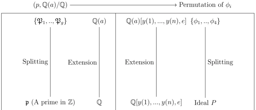
The situation emerging this computation would be illustrated by Fig.5.1. The Frobe-nius maps (p,Q(a)/Q) induces the permutation of the four quantum states{φi}. In other words, the Frobenius map in the underlying number fields induces the permutation of the prime ideals representing {φi} in the polynomial ring. For this reason, the conse-quence of class field theory in the underlying number fields emerges in the polynomial rings.
p (A prime in Z)
{P1, ..,Pg} Q(a)
Q
(p,Q(a)/Q) Permutation of φi
Q(a)[y(1), ..., y(n), e]
Q[y(1), ..., y(n), e] Ideal P
{φ1, .., φ4}
Splitting Extension Extension Splitting
Figure 5.1: The extension and the splitting in the computed model.
5.4
Chebotarev density theorem
LetL be the finite Galois extension of the number field K with the Galois group G. And let C be the subset of G stable under the conjugation. It has the following property: if σ ∈ C, τ ∈ G, then τ στ−1 ∈ G. (Usually,
C is called the conjugacy class.) Moreover, let T(C) be the set of prime ideals in K, being unramified prime in K, and accompanied by a certain type of Frobenius map such that (p, L/K)⊂C. EachT(C) shall occupy a certain amount of density in the infinite number of primes. This quantity is called the Dirichlet density. Then, according to the Chebotarev density theorem, the Dirichlet density forT(C) is related to two factors: the size of the conjugacy class and the order of the Group. It is given by the equation:
δ(T(C)) = #C #G
Note that this equation is not the definition; the left-hand side is the density of the subsets in the infinite number of primes, classified by the conjugacy classes; on the other hand, the right-side pertains to the Galois group; the relation between them is not trivial.
In the case of the model molecule with the Galois groupC2×C2(defined byha, b|a2=
b2 = 1, ab=bai), there are four types ofC[i] (i= 1,2,3,4), i.e.,
{{1},{a},{b},{ab}}.
As the group is abelian, each conjugacy class contains only one element and
δ(C[i]) = 1/4, for i = 1, ...,4.
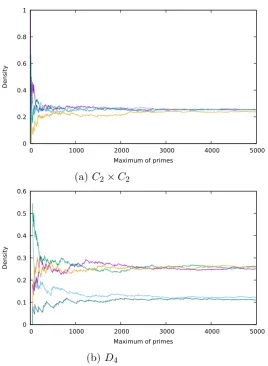
The numerical check verifies the statement. Using the finite set of primes (which contains every prime from 2 to a maximum, except those which ramify), one can compute the corresponding Frobenius elements, and evaluate the density for each conjugacy class. Fig. 5.2a is the plot of the variation of the densities of four Frobenius elements with the increase of the number of the sampled primes. Indeed, each density converges to 1/4. In the case of non-abelian extension, the density theorem is also valid. For the case of the model molecule with the Galois group D4, the definition of which is hr, s|r4 =s2 = 1,(rs)2= 1i. This group has five conjugacy classes:
{{1},{r2},{r, r3},{s, r2s},{rs, r3s}}.
These classes have the density
1/8,1/8,1/4,1/4,1/4,
0 0.2 0.4 0.6 0.8 1
0 1000 2000 3000 4000 5000
Density
Maximum of primes
(a) C2×C2
0 0.1 0.2 0.3 0.4 0.5 0.6
0 1000 2000 3000 4000 5000
Density
Maximum of primes
(b) D4
Figure 5.2: The numerical check of Chebotarev density theorem, using the com-putation of the model molecules: (a) the model with the Galois groupC2×C2; (b) the one with the Galois group D4. The densities are computed in the finite set of the first N primes (counted from 2). The vertical and the horizontal axis represent the density and the maximum one in the set of primes used in the estimation, respectively.